CH-DAV FP2020 (1997-2019)
This version is deprecated. An updated version of this dataset is available here: CH-DAV FP2022 (1997-2022.09)
Contents
Flux Products
- FP2020.1
Identifier: ID20201019114500
The original output fromReddyProcwith all NEE ustar scenarios (U05, U25, U50, U75, U95, ustar). - FP2020.2
Identifier: ID20201024221303
Output where some of the observed nighttime uptake after MDS gap-filling was corrected (U05, U25, U50, U75, U95). - FP2020.3 (recommended)
Identifier: ID20210502113257
Date: 3 May 2021
Added gap-filled fluxes for LE and ET, no other changes.
File:CH-DAV_FP2020.3_1997-2019_ID20210502113257_30MIN.csv
For an explanation of variables in the output file, please see here: ReddyProc Data Output Format
Description
PI flux product (FP) of Davos ecosystem flux and meteo data over 23 years between 1997-2019.
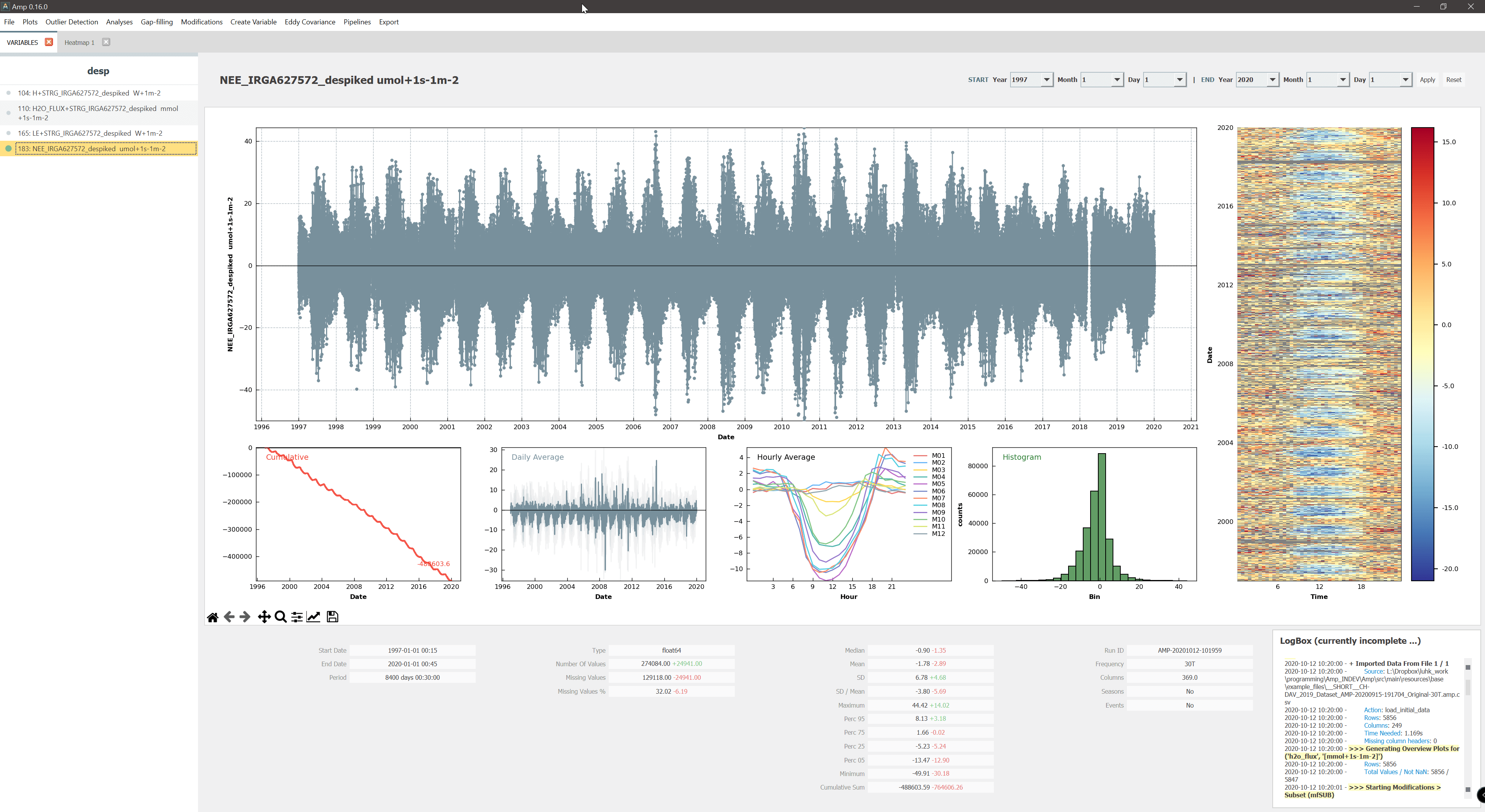
Different IRGAs were used to measure fluxes. The data of each IRGA were first merged into respective separate files that contained all Level-1 fluxes (the EddyPro output). Overall quality flags (QCF) were then calculated for each IRGA dataset, resulting in separate Level-2 datasets for each IRGA. These Level-2 datasets were then merged, resulting in continuous flux time series starting in Jan 1997 and ending in Dec 2019. The continuous NEE time series was then despiked, ustar filtered, gap-filled and partitioned into GPP and Reco, using the post-processing library ReddyProc (Link | Reference | Source Code), producing the flux product FP2020.1. Some time periods with strong nighttime uptake observed in this dataset after MDS gap-filling were corrected in FP2020.2.
During the earlier years 1997-2005, fluxes were measured using the closed-path IRGA LI-6262 (IRGA62), followed by measurements with the open-path IRGA LI-7500 (IRGA75) between 2005-2016. Recent years used the enclosed-path IRGA LI-7200 (IRGA72) between 2012-2019. During the overlapping IRGA75 / IRGA72 time periods, priority was given to the IRGA72 fluxes, while IRGA75 data (after corrections) was used to fill gaps in the IRGA72 time series.
The focus of this dataset is on the carbon fluxes, since the water fluxes during the earlier years 1997-2005 still need an additional correction. Nevertheless, energy fluxes LE and H were considered until incl. Step 7 (see below), but they were not gap-filled.
NEE fluxes were calculated for different ustar scenarios: U05, U25, U50, U75 and U95.
Recommended ustar scenario for NEE: U50, the median estimate of the ustar threshold (50% quantile of the bootstrapped uncertainty distribution).
For details about the correction and merging of different IRGA datasets please see below.
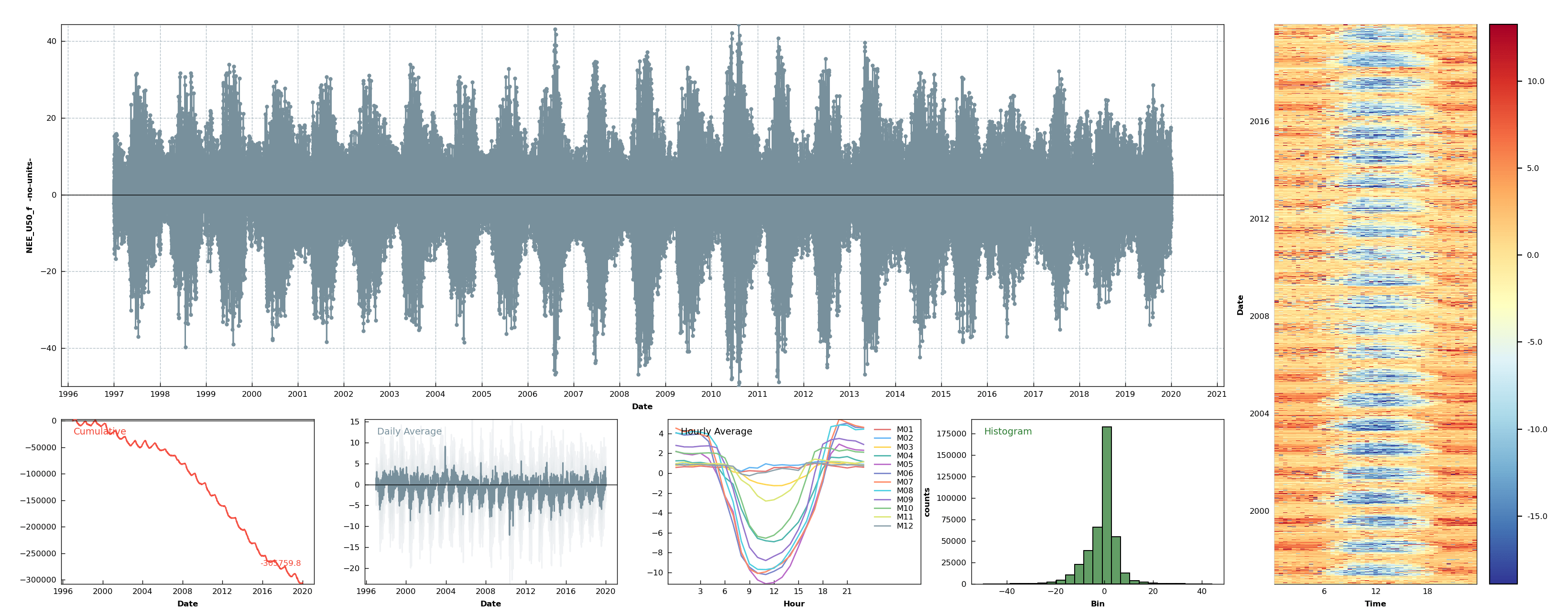
CH-DAV NEE 1997-2019 (NEE_U50_f from FP2020.2)
Key Stats
- Available measured values:
NEE_U50_f: 51.9% measured / 48.1% gap-filled (after all quality checks, outlier removal and ustar threshold application) - Range of U50 ustar thresholds: between 0.17 m s-1 (2008) and 0.33 m s-1 (2005), mean 0.24 m s-1 (1997-2019)
- Best estimate cumulative carbon uptake (1997-2019): 6.6 kg C m-2 (
NEE_U50_f), avg. 0.287 kg C m-2 yr-1 - Range cumulative carbon uptake in different ustar scenarios (1997-2019): between 4.7 kg C m-2 (
NEE_U95_f) and 9.2 kg C m-2 (NEE_U05_f) - Highest uptake 558 gC m-2 (2014)
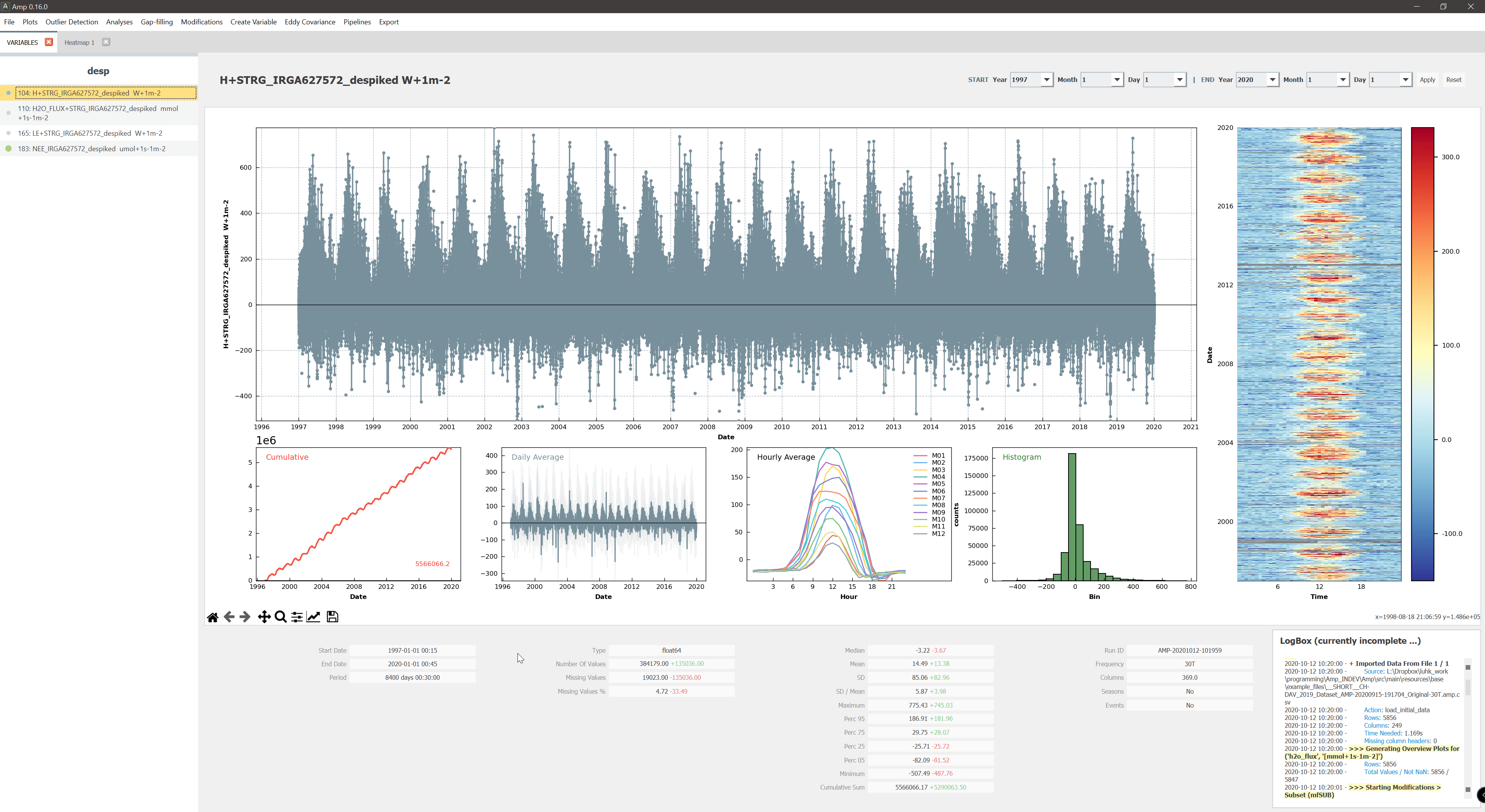
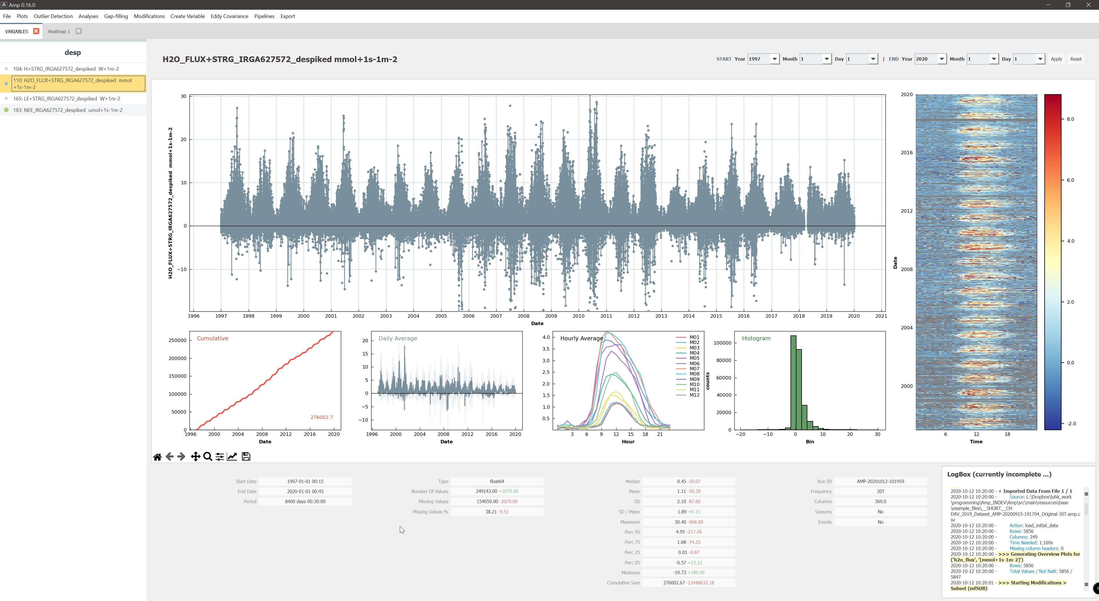
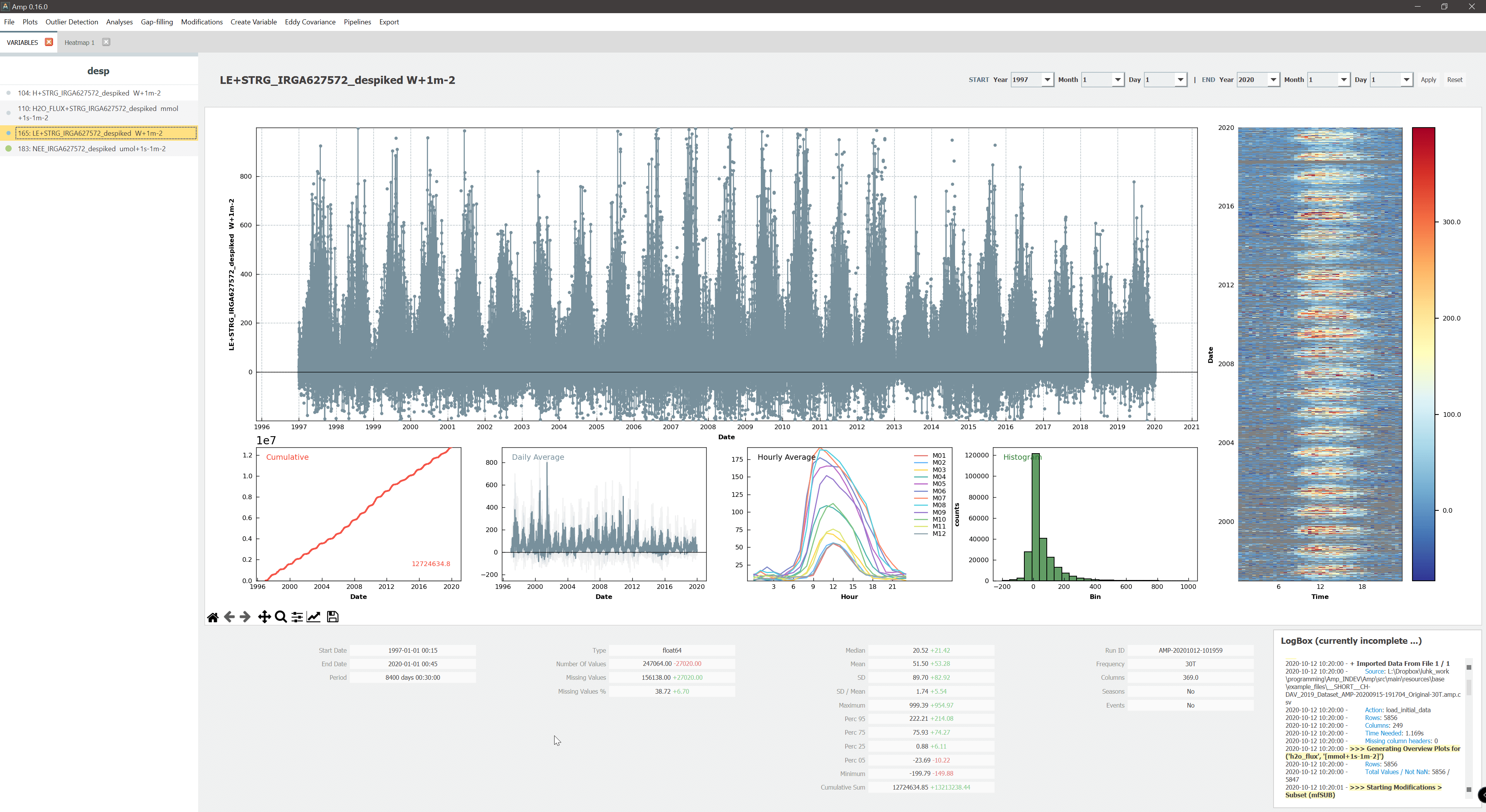
After Step 7, before ustar filtering
- Fluxes after application of quality flags (QCF) and after despiking.
- Missing data NEE: 32.0%
- Missing data LE: 38.7%
- Missing data H2O flux: 38.2%
- Missing data H: 4.7%
Dataset Production
Info about flux levels can be found here: Flux Levels
Software
EddyProfor flux calculations (links to details of Level-1 fluxes are given below for each year).ReddyProcfor ustar threshold detection, MDS gap-filliing and partitioning.DIIVE v0.16.0andv0.18.0for merging of data files, quality control, random forest gap-filling and the application of corrections (e.g. IRGA75 off-season uptake correction).
Setup
- Non-ICOS Setup 1997-2016 and ICOS Setup since 2014 (ETH binary files)
General Steps
Preparation of Level-2 Datasets
- STEP 1: LEVEL-1 COLLECTION: The most recent Level-1 fluxes for all IRGAs were collected.
- STEP 2: LEVEL-1 MERGING: Level-1 fluxes for each IRGA were merged.
- STEP 3: LEVEL-1 CORRECTIONS: Level-1 fluxes for IRGA75 were corrected for off-season uptake (XXX).
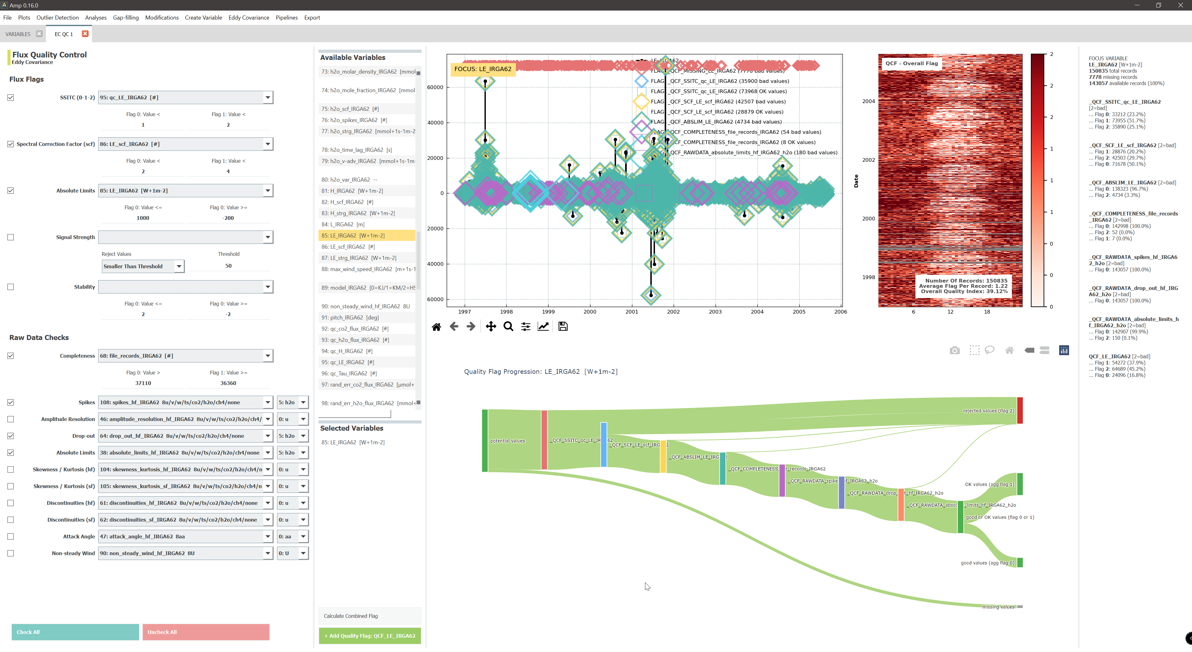
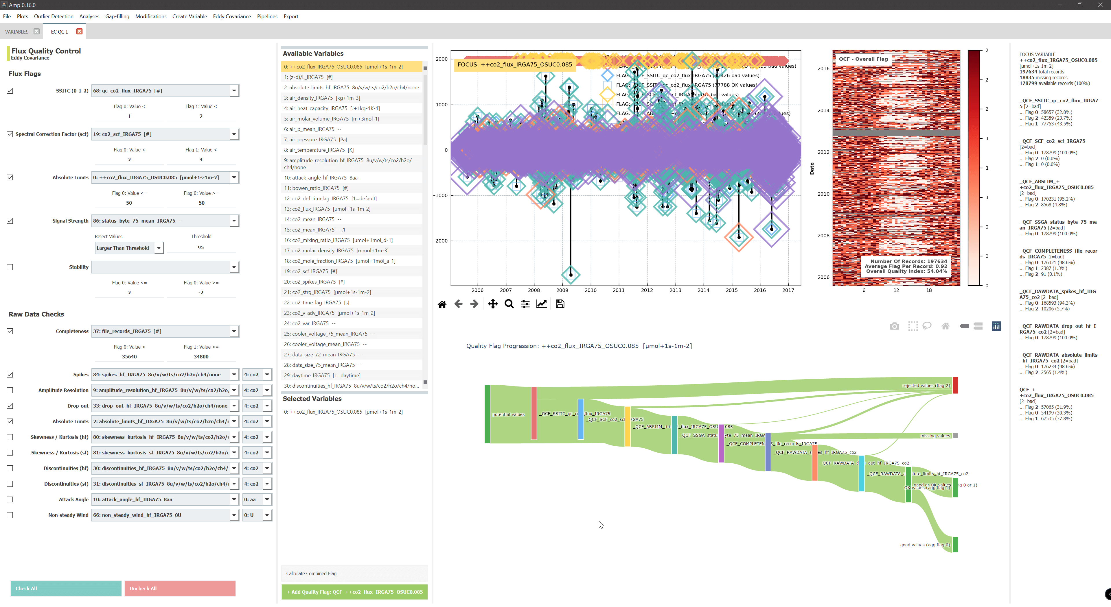
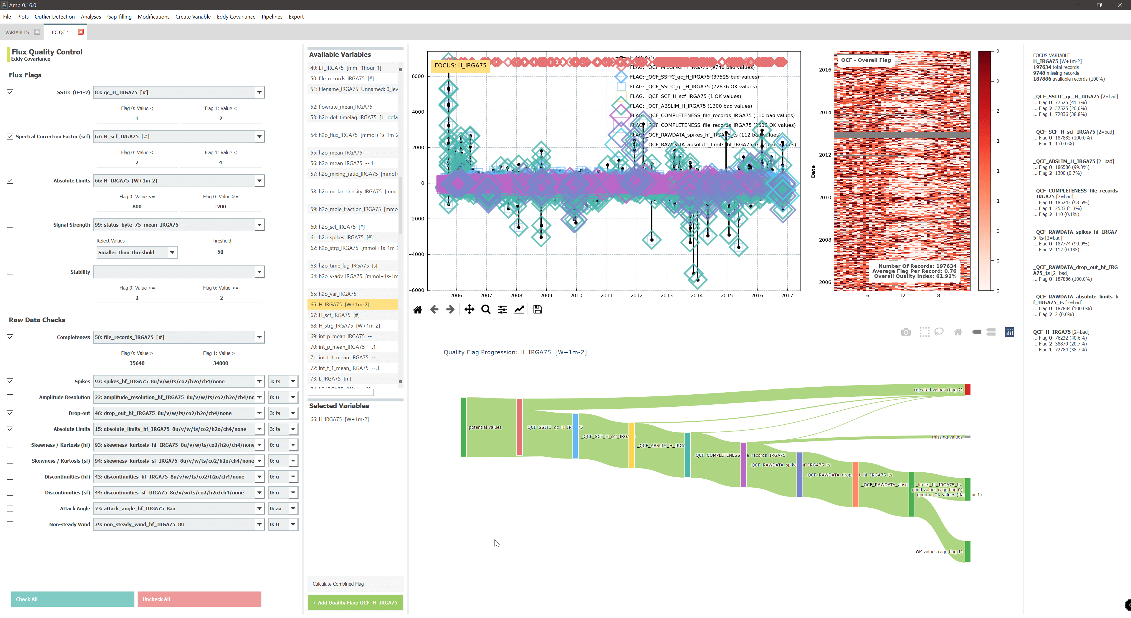
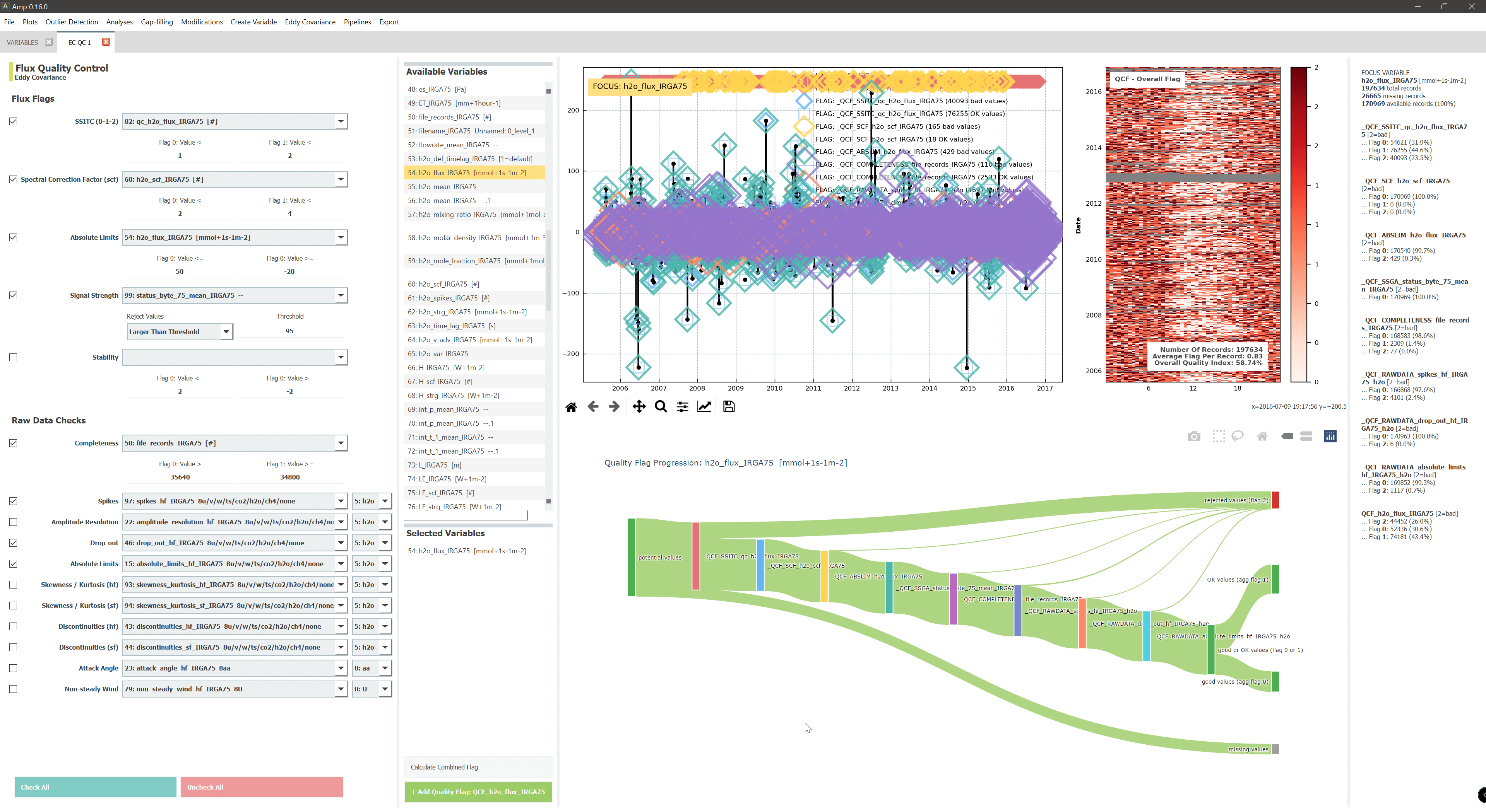
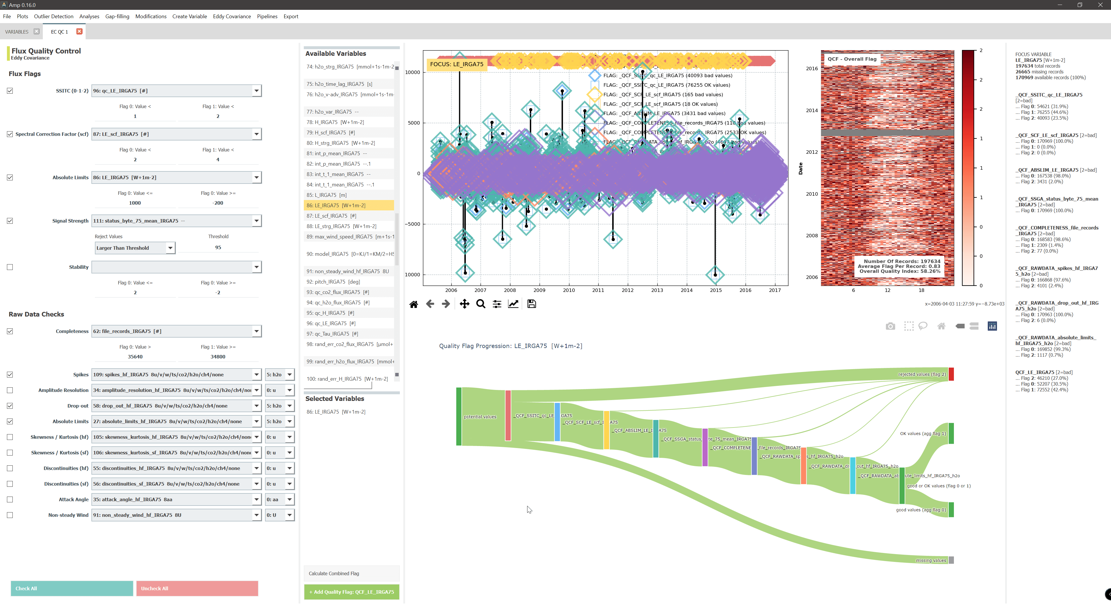
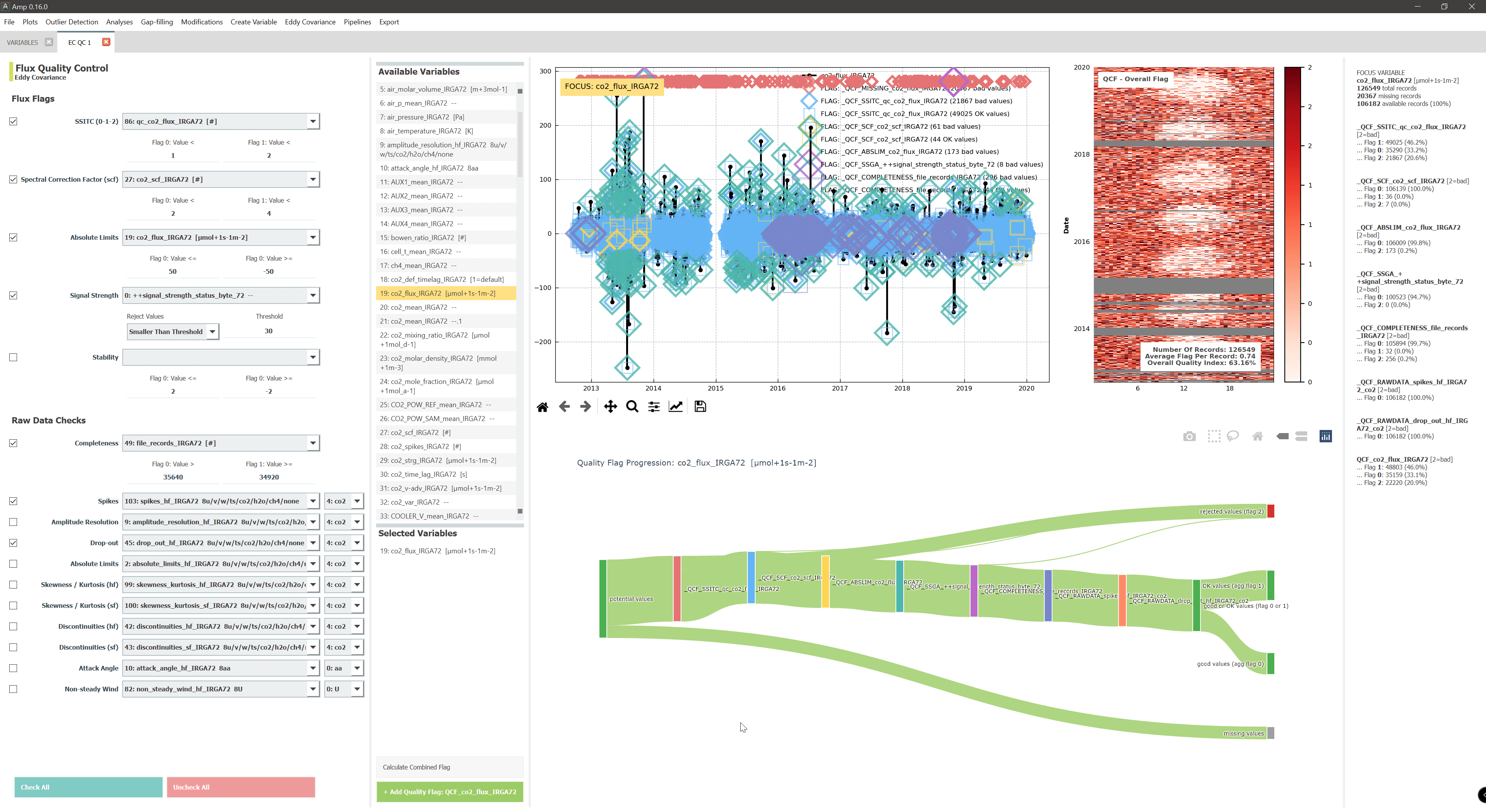
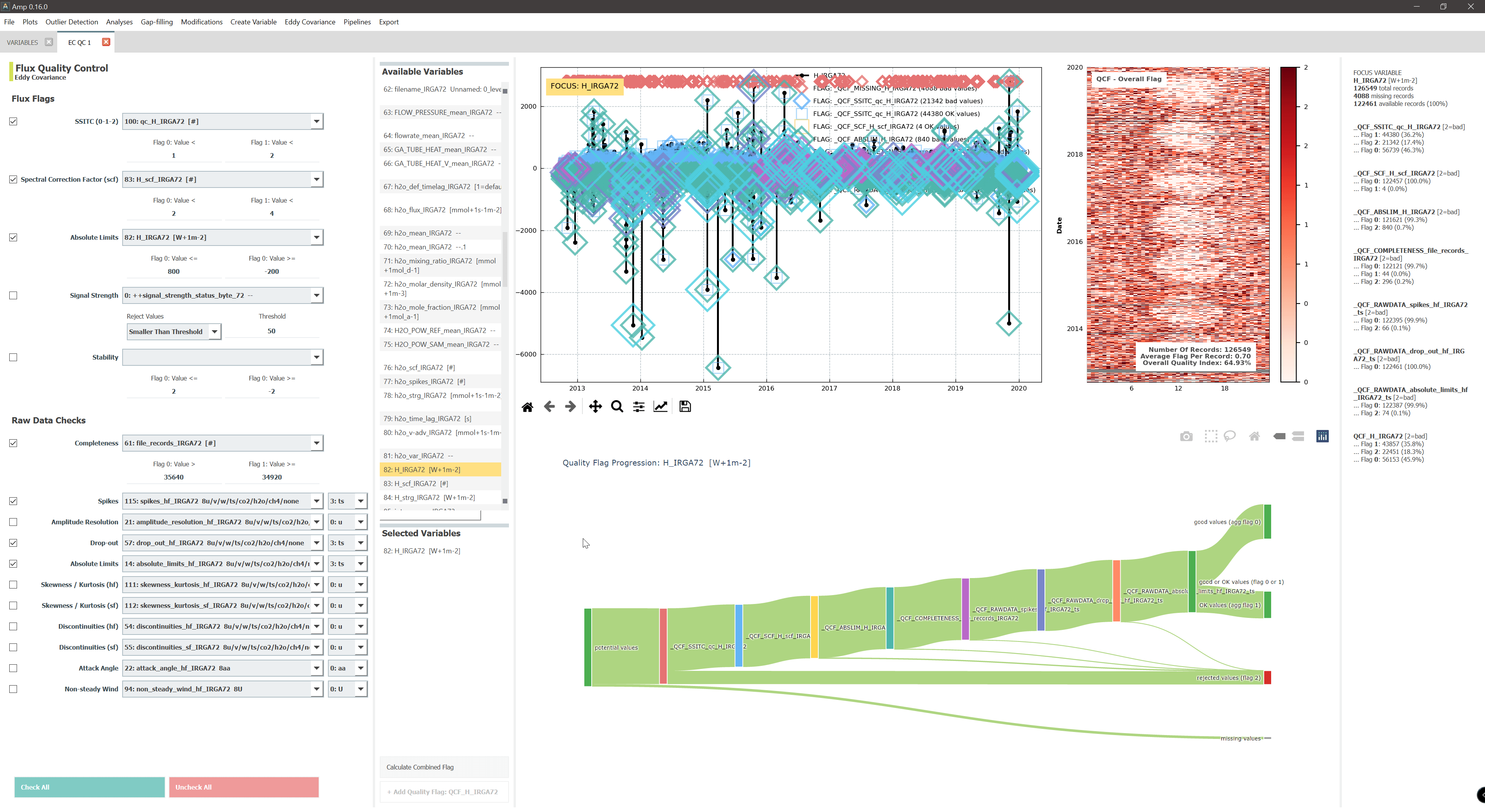
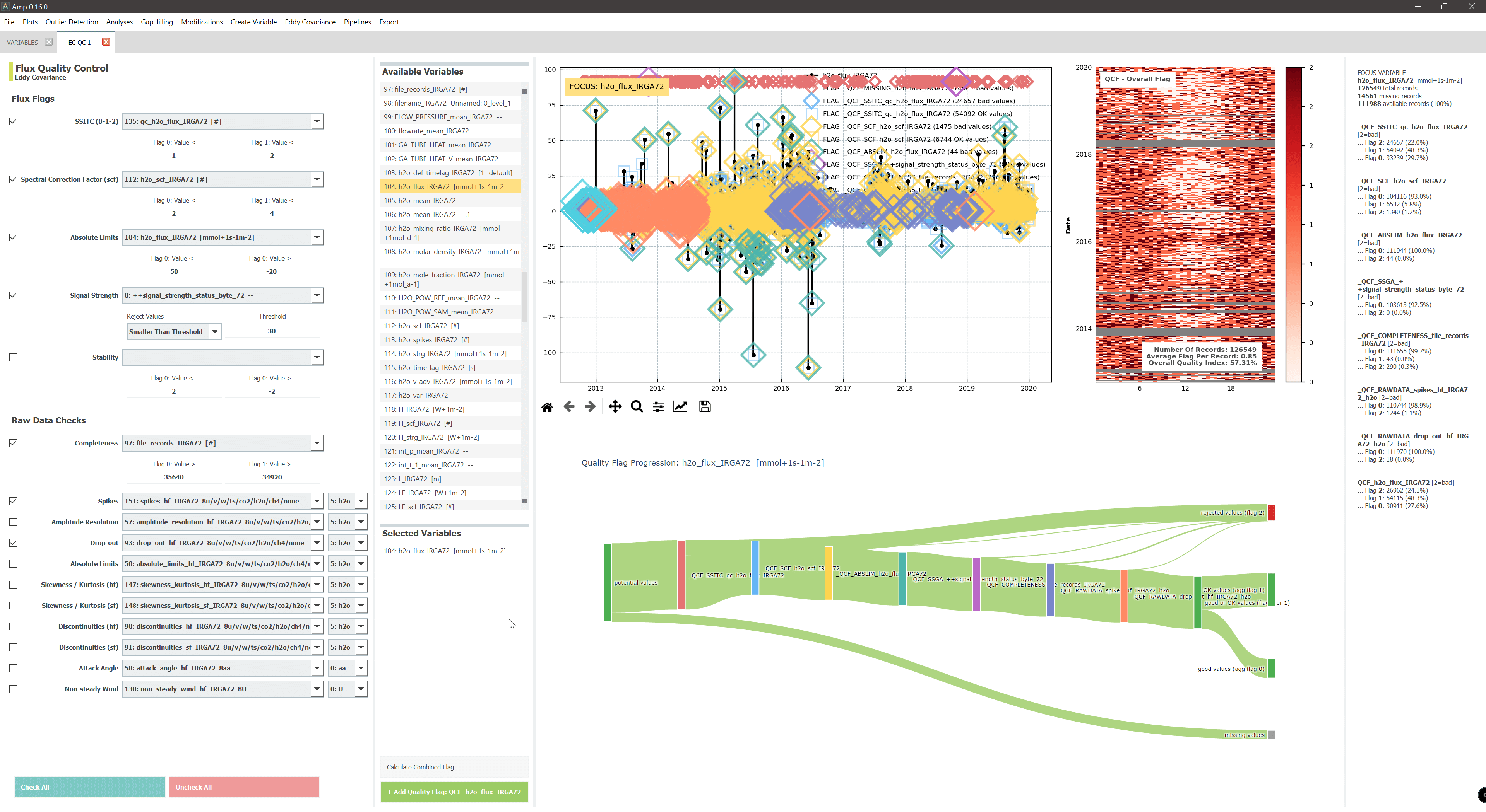
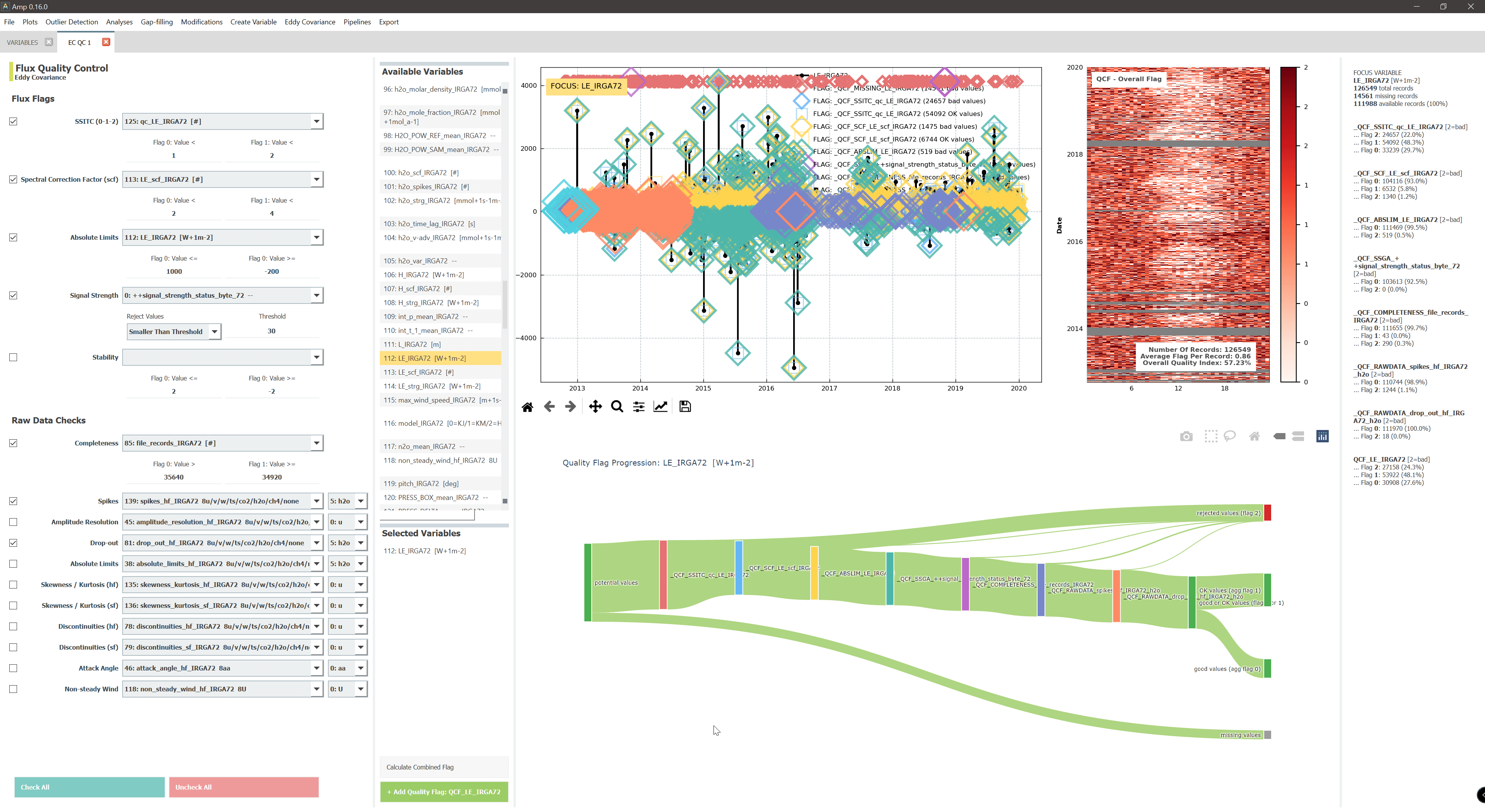
- STEP 4: LEVEL-2 QC: Level-2 fluxes (extended quality flags) were created for each IRGA, based on the merged dataset of the respective IRGA. QCF for fluxes: CO2, H2O, LE and H. For example, the quality flags for IRGA72 were created for all years from the merged IRGA72 dataset.
Prepare for ReddyProc Post-Processing
After Level-2, these additional steps prepared the data as input data for ReddyProc:
- STEP 5
- STORAGE CORRECTION: The storage term was added to CO2 flux, H2O flux, LE and H.
- QUALITY FLAG OVERLAPS: Only keep flux quality flags for which fluxes are available. This is necessary for the subsequent merging of different IRGA datasets, because each of these datasets also has a “missing” flag (flag 2) for flux values that are not available, but for successful merging datasets with real gaps where values are missing are needed.
- STEP 6
- MERGING: The different IRGA datasets were merged. As a result, e.g. all CO2 fluxes of all IRGAs were collected in one column. For this, the IRGA72 fluxes were used as the starting dataset. Then, IRGA62 fluxes were added (did not overlap with IRGA72 fluxes). Next, the IRGA75 fluxes were added, filling data gaps in the time series with IRGA75 values. Since there is an overlap between the measurements of the IRGA72 and IRGA75, this means that not only the IRGA75 data were added, but IRGA75 data were also used to fill data gaps in the IRGA72 time series, if possible. This was done not only for the fluxes, but also for the QCF data. This way all data points should have their respective correct data flag, even though there is this mixing of IRGAs with sometimes different QCF criteria.
- STEP 7
- QCF APPLICATION: Bad values (flag = 2) were removed from CO2 flux, H2O flux, LE and H.
- OUTLIER REMOVAL: CO2 flux, H2O flux, LE and H were despiked using the approach described in Papale et al. (2006). In addition a running median filter (centered) in a time window of 1440 records (30 days) and a SD range multiplier of 4-7 was applied, depending on the severity of some of the outliers. The running median filter was sometimes slightly adjusted in case severe outliers were still present in the dataset, e.g. the H2O fluxes for the open-path IRGA75 were generally characterized by more spikes than the data from IRGA62 and IRGA72, and the median filter was adjusted to catch some of the most extreme outliers. In this case, the time window was reduced to 720 records (15 days) with the SD range multiplier of 6-7.
- STEP 8
- Subset for subsequent post-processing steps ustar filtering, gap-filling and partitioning in
ReddyProc. - Subset only contain NEE, LE and their respective quality flags (QCF), and ustar.
- Subset for subsequent post-processing steps ustar filtering, gap-filling and partitioning in
Post-processing NEE
- STEP 9
- creates
FP2020.1 - done using
ReddyProc - (9.1) USTAR FILTERING: annual thresholds, only for NEE (Papale et al., 2006; Wutzler et al., 2018), USTAR scenarios: U05, U25, U50, U75, U95 (all bootstrapped 200x) and ustar (not bootstrapped)
- (9.2) GAP-FILLING: MDS (Reichstein et al., 2005)
- (9.3) PARTITIONING: nighttime partitioning (Reichstein et al., 2005)
- BEST ESTIMATE NEE:
NEE_U50_f - Done in
CH_DAV_FP2020.1_30min_GapFilledPartitionedFluxes_ID20201019114500.csv
- creates
Post-processing Corrections NEE
- The MDS gap-filling algorithm produced some unusual nighttime CO2 uptake because during the respective time periods mostly measured data that showed uptake during nighttime were available for the look-up table.
- The nighttime uptake due to gap-filling is potentially wrong and was correctected in
FP2020.2. - Nighttime uptake was observed for the following time periods:
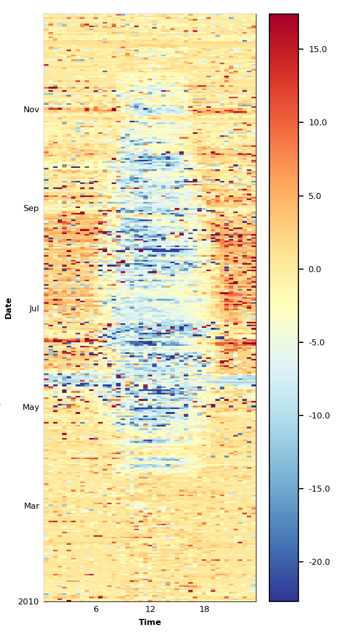
- 5 May – 23 May 2010 (19 days, see Figure 11.3)
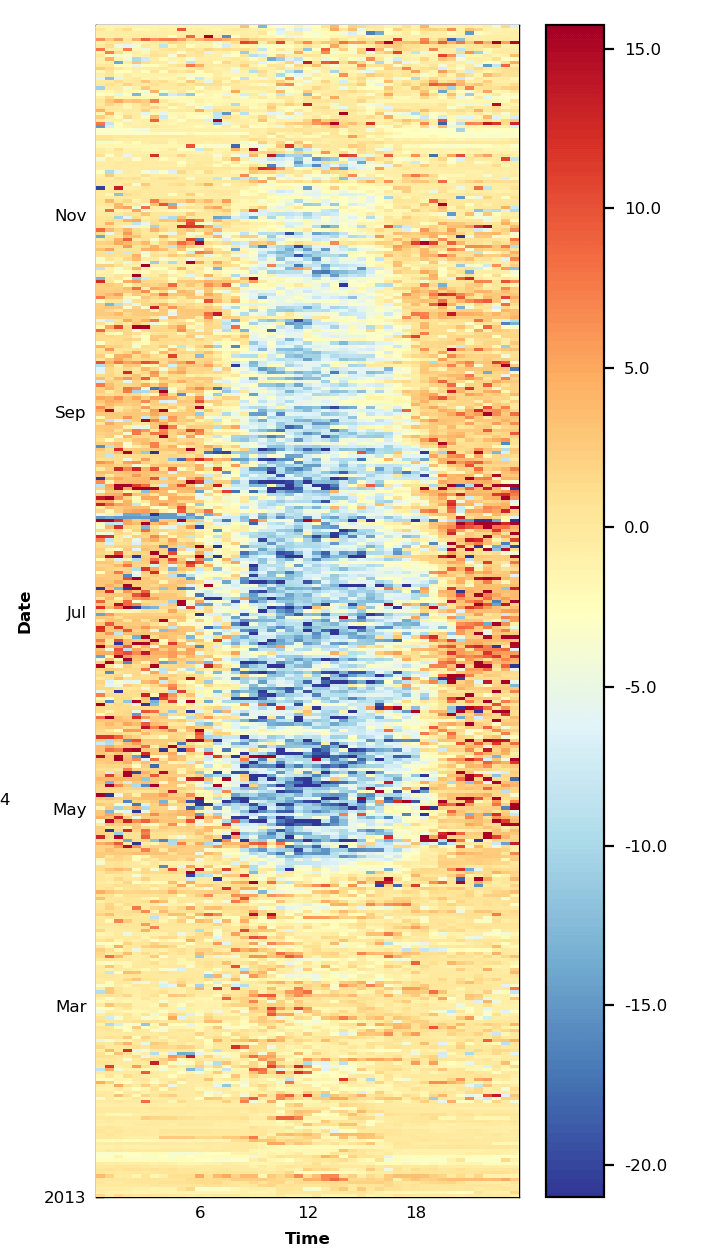
- 29 July – 31 July 2013 (3 days)
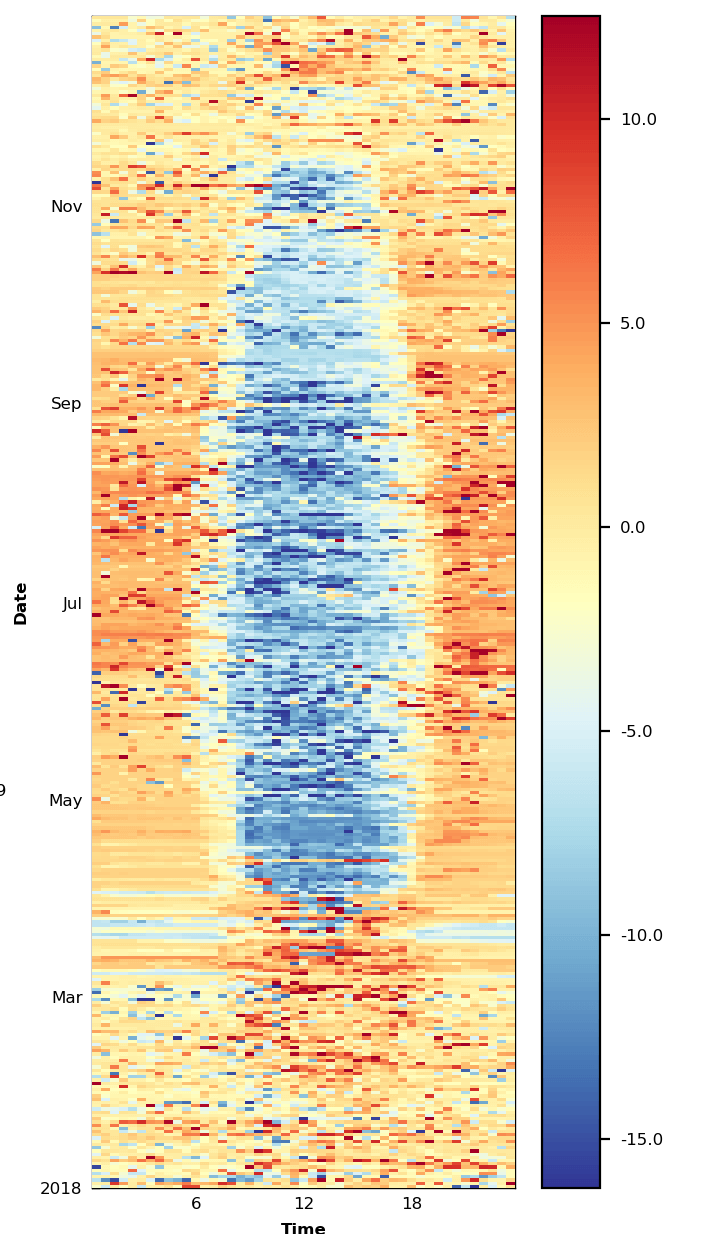
- 18 March – 25 March 2018, during the large data gap (8 days)
- 2 April 2018 (1 day)
- Here are the time periods in question from an earlier run, but the same time periods showed uptake also in the final run:
- STEP 10
- (10.1) GAP-FILLING: the different USTAR scenarios from Step (9.1) (U05, U25, U50, U75, U95) were gap-filled with random forest using TA, SW_IN and VPD, using
DIIVEv0.16.0 - (10.2) PARTITIONING: nighttime partitioning for each USTAR scenario (Reichstein et al., 2005) in
ReddyProc - (10.3) MERGING: all USTAR scenarios were merged into one file
- (10.1) GAP-FILLING: the different USTAR scenarios from Step (9.1) (U05, U25, U50, U75, U95) were gap-filled with random forest using TA, SW_IN and VPD, using
- STEP 11
- creates
FP2020.2 - (11.1) REMOVAL of nighttime uptake periods from all variables from Step (9.3)
- (11.2) GAP-FILLING the flux gaps created in Step (11.1) with the gap-filled values from Step (10.3)
- (11.3) GAP-FILLING the all other gaps created in Step (11.1) with the original
FP2020.1values.
- creates
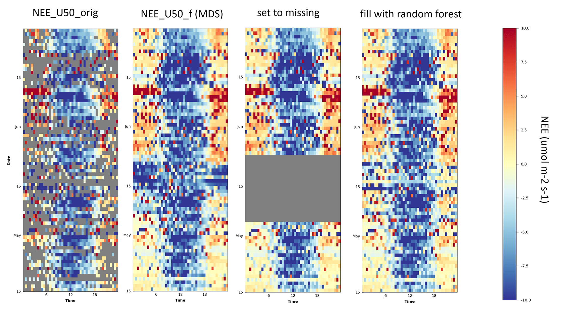
Figure 11.3: CH-DAV 2010: Example for replacement of MDS gap-filled values with values from random forest gap-filling in FP2020.2. During the corrected time period, originally measured values were kept, but MDS gap-filled values were substituted with random forest gap-filled values. This was done because during some time periods the MDS gap-filling resulted in relatively strong nighttime CO2 uptake. Note that in this example some measured nighttime uptake passed all quality checks and therefore remained in the dataset. Due to these values, MDS filled missing gaps with mostly uptake (fill quality=1, i.e. highest quality), while this effect was less pronounced in random forest.
- STEP 12
- add additional fluxes to the dataset: LE and ET
- (12.1) GAP-FILLING flux LE from Step 8 was gap-filled using the MDS method with SW_IN, TA and VPD
- (12.2) CALCULATE ET from gap-filled LE. Since ET is the same flux with different units as LE, it was calculated in
ReddyProc. - Done in
CH_DAV_30min_LE_ET_GapFilled_ID20210502223451.csv
- STEP 13
- creates
FP2020.3 - merging gap-filled LE and ET with FP2020.2
- Done in
CH-DAV_FP2020.3_1997-2019_ID20210502113257_30MIN.csv
- creates
Details
1997-2005: R2-IRGA62
STEP 1 – COLLECTION
- 1997 R2-IRGA62_FF-201606 / Level-1_ID2016-07-27T220640
- 1998 R2-IRGA62_FF-201606 /Level-1_ID2016-07-27T220629
- 1999 R2-IRGA62_FF-201606 /Level-1_ID2016-07-27T220619
- 2000 R2-IRGA62_FF-201606 /Level-1_ID2016-07-27T220606
- 2001 R2-IRGA62_FF-201606 /Level-1_ID2016-07-27T221217
- 2002 R2-IRGA62_FF-201606 /Level-1_ID2016-07-27T220552
- 2003 R2-IRGA62_FF-201606 /Level-1_ID2016-07-27T220527
- 2004 R2-IRGA62_FF-201606 /Level-1_ID2016-07-27T220516
- 2005 R2-IRGA62-IRGA75_FF-201606 /Level-1_ID2016-07-28T143836 IRGA62 fluxes only
STEP 2 – MERGING
- Merged dataset:
1997-2005_IRGA62_Level-1_Dataset_AMP-20201006-151801_Original-30T.amp.csv
STEP 3 – CORRECTIONS
- Exclusion: CO2 flux data between 27 Feb 2001 and incl. 23 Mar 2001 was excluded from the dataset. See here for more information: CH-DAV: 2001
STEP 4 – QC
- Merged dataset with QCF:
1997-2005_IRGA62_Level-2_Dataset_AMP-20201010-224852_Original-30T.amp.csv
STEP 5 – ADD STORAGE AND QC FLAG OVERLAPS
- Done in
1997-2005_IRGA62_Dataset_AMP-20201011-224422_Original-30T.amp.csv
2005-2016: R2-IRGA75
STEP 1 – COLLECTION
Important: Level-1 fluxes for the IRGA75 are not corrected for off-season uptake (Burba et al.).
- 2005 R2-IRGA62-IRGA75_FF-201606 / Level-1_ID2016-07-28T143836
- 2006 R2-R350-IRGA75_FF-201606 / Level-1_ID2016-06-03T151158
- 2007 R350-IRGA75_FF-201606 / Level-1_ID2016-06-01T145942
- 2008 R350-IRGA75_FF-201606 / Level-1_ID2016-05-30T161917
- 2009 R350-IRGA75_FF-201606 / Level-1_ID2016-05-30T161726
- 2010 R350-IRGA75_FF-201606 / Level-1_ID2016-05-29T160744
- 2011 R350-IRGA75_FF-201606 / Level-1_ID2016-05-29T160603
- 2012_1 R350-IRGA75_FF-201606 / Level-1_ID2016-06-06T173342
- 2013_2 R350-IRGA75_FF-201606 / Level-1_ID2016-05-31T124327
- 2014 R350-IRGA75_FF-201606 / Level-1_ID2016-05-31T122130
- 2015 R350-IRGA75_FF-201606 / Level-1_ID2016-05-31T155418
- 2016 R350-IRGA75_FF-201909 / Level-1_ID2019-09-23T195556_noBurba
STEP 2 – MERGING
- Merged dataset:
2005-2016_IRGA75_Level-1_Dataset_AMP-20201006-151801_Original-30T.amp.csv
STEP 3 – CORRECTIONS
- CO2 fluxes in the merged dataset were corrected for off-season uptake before calculating QCF (Burba et al., 2008). The correction was applied with a correction factor of 8.5% (Järvi et al., 2009). I compared time periods during which both IRGA72 and IRGA75 fluxes were available. The 8.5% correction factor was selected as a compromise and yielded IRGA75 fluxes that were more comparable / more similar to the concurrently measured IRGA72 fluxes. However, during certain time periods a lower correction factor would have been more accurate, but overall the 8.5% factor yielded satisfactory results. In the future, this issue will be re-visited to find a solution that is as optimal as possible.
STEP 4 – QC
- Merged dataset with QCF:
2005-2016_IRGA75_Level-2_Dataset_AMP-20201010-224852_Original-30T.amp.csv
STEP 5 – ADD STORAGE AND QC FLAG OVERLAPS
- Done in
2005-2016_IRGA75_Dataset_AMP-20201011-141659_Original-30T.amp.csv
2012-2019: R350-IRGA72 and HS50-IRGA72
STEP 1 – COLLECTION
- 2012_2 R350-IRGA75_FF-201606 / Level-1_ID2016-06-06T173342 contains IRGA72 fluxes
- 2013 R350-IRGA72_FF-201909 / Level-1_ID2019-09-23T195553
- 2014 R350-HS50-IRGA72_FF-201909 / Level-1_AMP-20190927-122651
- 2015 HS50-IRGA72_FF-202008 / Level-1_ID2020-08-15T224409
- 2016 HS50-IRGA72_FF-201902 / Level-1_ID2019-02-25T194303
- 2017 HS50-IRGA72_FF-201902 / Level-1_ID2019-02-25T202725
- 2018 HS50-IRGA72_FF-201902 / Level-1_ID2019-03-02T164252
- 2019 HS50-IRGA72_FF-202005 / Level-1_ID2020-05-22T122418
STEP 2 – MERGING
- Merged dataset:
2012-2019_IRGA72_Level-1_Dataset_AMP-20201006-112042_Original-30T.amp.csv
STEP 3 – CORRECTIONS
- –
STEP 4 – QC
- Note about IRGA72 signal strength: In the Level-1 files, the signal strength was still called
status_bytein the earlier IRGA72 flux calculations until approx. end of 2014. As far as I remember, during these earlier years the given number represents good signal strength when the number is low, and bad signal strength if the number is high (see Figure below). After a IRGA software update, this convention was inversed, meaning that after the update a high number means good signal, and a low number means bad signal. This change in convention makes it impossible to quality control all merged IRGA72 results in the same run. However, after checking the data it seems clear that there was no major issue with signal strength in 2013 and 2014. Therefore, all IRGA72 data (status_byte_72andsignal_strength_72) were merged and values below a very low threshold (30) were rejected. This low threshold is below a realistic value also for the 2013-2014 years, so that the fluxes are not impacted negatively by this flag.
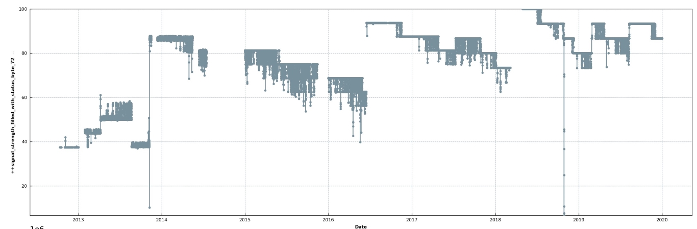
CH-DAV IRGA72 signal strength and status byte values between 2013 and 2019.
- Note about the raw data check for absolute limits: This QC test was deactivated because it resulted in a considerable data loss during approx. two years. Fluxes during the respective time period looked good.
- Merged dataset with QCF:
2012-2019_IRGA72_Level-2_Dataset_AMP-20201010-224852_Original-30T.amp.csv
STEP 5 – ADD STORAGE AND QC FLAG OVERLAPS
- Done in
2012-2019_IRGA72_Dataset_AMP-20201011-141659_Original-30T.amp.csv
Known Issues
- Water fluxes 1997-2005 are underestimated in this dataset and still need an additional correction. This issue will be addressed in detail in one of the next flux products.
- The off-season uptake correction needed for IRGA75 CO2 fluxes is not perfect (it never is…), but the applied correction yielded fluxes that were more similar to overlapping IRGA62 and IRGA72 fluxes. Without this correction, IRGA75 fluxes clearly showed off-season uptake rates that were too high.
- Unfortunately there are no time periods of overlapping IRGA62 and IRGA75 / IRGA72 measurements. It is therefore difficult to say how comparable these fluxes are to later years and if they need an additional correction. This issue will be re-visited in the future.
- Nighttime NEE in the early years (1997-2005) seems to be overestimated (too much emission) in comparison to all other years. This could be due to an issue during calibration of the LI-6262 (chemicals? Not clear from the documentation). This issue will be revisited in the future.
- The wind direction calculation for most of the years is slightly wrong. We found out about this issue during the ICOS labelling process and old flux calculations were not corrected retroactively. The correct wind direction was calculated (at least) for 2019. In comparison to most previous years the wind direction in 2019 was approx. -20°. If the correct wind direction for the other years should be needed, it can be corrected by subtracting the degrees from the wind direction output. This issue will be corrected in the next PIDS.
References
- Burba, G. G., McDERMITT, D. K., Grelle, A., Anderson, D. J., & Xu, L. (2008). Addressing the influence of instrument surface heat exchange on the measurements of CO 2 flux from open-path gas analyzers. Global Change Biology, 14(8), 1854–1876. https://doi.org/10.1111/j.1365-2486.2008.01606.x
- Järvi, L., Mammarella, I., Eugster, W., Ibrom, A., Siivola, E., Dellwik, E., Keronen, P., Burba, G., & Vesala, T. (2009). Comparison of net CO2 fluxes measured with open- and closed-path infrared gas analyzers in an urban complex environment. 14, 16.
- Papale, D., Reichstein, M., Aubinet, M., Canfora, E., Bernhofer, C., Kutsch, W., Longdoz, B., Rambal, S., Valentini, R., Vesala, T., & Yakir, D. (2006). Towards a standardized processing of Net Ecosystem Exchange measured with eddy covariance technique: Algorithms and uncertainty estimation. Biogeosciences, 3(4), 571–583. https://doi.org/10.5194/bg-3-571-2006
-
Reichstein, M., Falge, E., Baldocchi, D., Papale, D., Aubinet, M., Berbigier, P., Bernhofer, C., Buchmann, N., Gilmanov, T., Granier, A., Grunwald, T., Havrankova, K., Ilvesniemi, H., Janous, D., Knohl, A., Laurila, T., Lohila, A., Loustau, D., Matteucci, G., … Valentini, R. (2005). On the separation of net ecosystem exchange into assimilation and ecosystem respiration: Review and improved algorithm. Global Change Biology, 11(9), 1424–1439. https://doi.org/10.1111/j.1365-2486.2005.001002.x
- Wutzler, T., Lucas-Moffat, A., Migliavacca, M., Knauer, J., Sickel, K., Šigut, L., Menzer, O., & Reichstein, M. (2018). Basic and extensible post-processing of eddy covariance flux data with REddyProc. Biogeosciences, 15(16), 5015–5030. https://doi.org/10.5194/bg-15-5015-2018
Last Updated on 5 Oct 2024 13:20