CH-DAV FP2022 (1997-2022)

STATUS: Released.

Flux Products

For a description of variables in output files, please see Variable Abbreviations and ReddyProc Data Output Format

Current Version

FP2022.5 (recommended)

• Date: 6 Feb 2023
  
• Identifier: ID20230206154316
• Files:
  • CH-DAV_FP2022.5_1997-2022_ID20230206154316_30MIN.csv (timestamp shows END)
  • CH-DAV_FP2022.5_1997-2022_ID20230206154316_30MIN.diive.csv (same data, but timestamp shows MIDDLE)
  • CH-DAV_FP2022.5_1997-2022_ID20230206154316_30MIN_list_of_variables_and_units.csv (List of variables and their units)
• Description:
  • PI flux dataset using a constant USTAR threshold for all years (CUT = 0.287644), MDS gap-filling and partitioning done in ReddyProc
• Difference to FP2021.2:
  • Years 2021 (complete) and 2022 (complete) have been added.
  • Additional meteo data
• Difference to FP2022.4:
  • Complete year 2022 is now included
• Included variables: NEE, GPP, Reco, TA, SW_IN, VPD, PPFD, RH, LW_IN, PA, PREC, SWC (1 depth at 1 location) and auxiliary output
• Recommended flux variables:
  • Gap-filled: NEE_CUT_REF_f, LE_f, ET_f, GPP_ and RECO_ from daytime (Lasslop et al., 2010) and nighttime (Reichstein et al., 2005) partitioning
  • To obtain measured only (not gap-filled) highest quality fluxes use:
    • NEE_CUT_REF_orig where the respective quality flag QCF_NEE = 0
    • LE_orig where the respective quality flag QCF_LE = 0

Deprecated Versions

FP2022.4 (deprecated)

• Date: 4 Dec 2022 / Identifier: ID20221204161958
• Difference to FP2021.2:
  • Years 2021 (complete) and 2022 (until 30 September) have been added.
  • Additional meteo data
• Difference to FP2022.3:
  • Corrected values since 16 Jul 2019 for precipitation PREC_TOT_T1_25+20_1, the previous precipitation PRECIP has been removed
  • Units are now included in the .diive.csv file

FP2022.3 (deprecated)

• Date: 28 Oct 2022 / Identifier: ID20221028163633
• Difference to FP2021.2:
  • Years 2021 (complete) and 2022 (until 30 September) have been added.
  • Additional meteo data
• Difference to FP2022.2:
  • Added meteo variables PRECIP (precipitation) and SWC_FF0_0.15_1

FP2022.2 (deprecated)

• Date: 23 Oct 2022 / Identifier: ID20220826234456
• Difference to FP2021.2:
  • Years 2021 (complete) and 2022 (until 30 September) have been added.
• Difference to FP2022.1:
  • Data 2022 (until 30 September) have been added.
  • More meteo variables are included.

FP2022.1 (deprecated)

• Date: 26 Aug 2022 / Identifier: ID20220826234456
• Difference to FP2021.2 (previous version):
  • Years 2021 (complete) and 2022 (until 11 August) have been added.

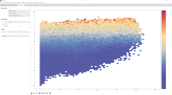
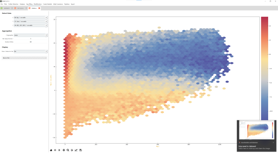
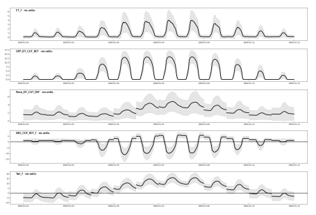
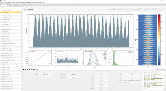
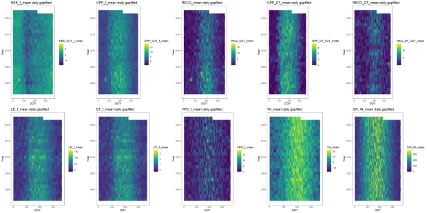
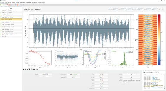
Plots

Plots show the time range 1997-2022.08 from FP2022.1 (until 11 Aug 2022)

Description

• Ecosystem fluxes over 26 years from three different IRGAs and sonic anemometers
• This is the third version of the CH-DAV PI dataset. The first version can be found here, but note the differences in post-processing. The second version can be found here.
• Important notes:
  • Usage of a constant USTAR threshold, same across years (before: separate, variable USTAR thresholds for each year)
  • Gap-filled NEE data was calculated from daytime NEE data with quality flags 0 and 1, and from nighttime NEE data with quality flag 0 (highest quality) (before: also nighttime NEE of quality 1 were included)
  • Due to the use of highest quality nighttime fluxes there are many gaps to be filled during nighttime, and nighttime respiration in gap-filled NEE is significantly higher than in the very first version of this dataset (FP2020).
  • The IRGA75 middle years (2005-2016) were corrected for self-heating using a refined approach similar to Kittler et al. (2017). This increased nighttime respiration, while daytime fluxes remained mostly unchanged (minor differences to before).
  • Calculated budgets are now closer to the FLUXNET estimates

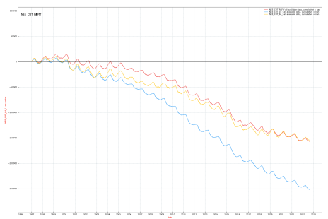
Key Stats

From FP2022.1 (without year 2022):

• Best estimate cumulative carbon uptake (1997-2021): 3.3 kg C m-2 (NEE_CUT_REF_f), avg. 133 g C m-2 yr-1
  • The partly included year 2022 (until 30 Sep) was not included in this estimate.
• Available directly measured, highest-quality fluxes:
  • directly measured fluxes with quality flag QCF = 0 (no gap-filling)
  • NEE_CUT_REF_orig_QCF0: 96741 values (22.1% of potential values) [1], [2], [3]
  • LE_orig_QCF0: 102103 values (23.3% of potential values) [1], [3]
  • ET_f_QCF0: 103564 values (23.6% of potential values) [1], [3]
• Data basis for budget calculations:
  • NEE_CUT_f: 30.2% measured / 69.8% gap-filled [1], [2], [4] (calculated from NEE_CUT_REF_orig)
  • LE_f and ET_f: 60.4% measured / 39.6% gap-filled [1], [5] (calculated from LE_orig)

[1] … after all quality checks, including outlier removal
[2] … after USTAR threshold application
[3] … QCF = 0 (daytime and nighttime)
[4] … measured data include quality flag QCF = 0 and QCF = 1 (OK quality) for daytime data, and QCF = 0 for nighttime data
[5] … measured data include quality flag QCF = 0 and QCF = 1 for daytime and nighttime data

Dataset Production

Software

• EddyPro v6 and v7 for flux calculations (links to details of Level-1 fluxes are given below for each year)
• bico for the conversion of binary raw data files to ASCII (2013-2016, 2020-2022)
• fluxrun for the flux calculation using EddyPro (2013-2016, 2020-2022)
• Various versions of FCT (flux calculation using EddyPro) were used for years 1997-2004 and 2017-2019, details are given in the section Used Flux Versions below
• scop v0.1 (self-heating correction for open-path IRGAs) for the self-heating correction of IRGA75 fluxes
• diive v0.21.0 (legacy version) for file merging, quality control, storage correction, outlier removal
• ReddyProc v1.2.2 for application of the constant ustar threshold, MDS gap-filliing and partitioning, in R Studio v1.3.959

Flux calculations

• Some important processing steps for the calculation of Level-1 fluxes
• For info about the flux processing chain and flux levels see: Flux Processing Chain
• Flux calculations were done using EddyPro v6 and v7, using the Python wrapper fluxrun or its predecessor FCT. Both wrappers are running EddyPro in the background but provide additional output.
• Statistical analysis
  • Statistical tests for raw data screening (Vickers and Mahrt, 1997) for all IRGAs: spike count/removal, drop-outs, absolute limits
• Axis rotation for tilt correction: double rotation
• Turbulent fluctuations: Detrend method: Block average
• Compensation of density fluctuations
  • Open-path IRGA75 fluxes (2005-2016) were compensated for density fluctuations (WPL terms) (Webb, Pearman and Leuning, 1980)
  • For the correction of the IRGA75 self-heating effect, see notes on Level-1.1 below. The self-heating effect was not corrected in EddyPro because IRGAs at CH-DAV are tilted (15°) and the implemented correction was developed for vertically-mounted instruments.
• Time lag determination
  • Time lag was first determined in a time window of 0-10s
  • The distribution of found lags was investigated in histograms
  • The peak distribution was used as the nominal/default time lag
  • During the calculation of Level-1 fluxes, the time window 0-10s was used, with the nominal time lag used for half-hours where no clear time lag was found
  • Early years 1997-2005 used the automatic time lag optimization as implemented in EddyProwhich follows a similar approach
• Spectral correction
  • High frequency range / correction of low-pass filtering effects:
    • Horst (1997) for closed-path IRGA62 fluxes (1997-2005)
    • Horst (1997) for open-path IRGA75 fluxes (2005-2016)
    • Fratini et al. (2012) for enclosed-path IRGA72 fluxes (2012-2022)
  • Low frequency range:
    • Analytic correction of high-pass filtering effects (Moncrieff et al., 2004) for all IRGAs

Flux post-processing

For an overview of the general processing chain see here: Flux Processing Chain

Steps to create a flux dataset comprising CO2 flux (NEE), LE and H. Note that H2O flux and ET are not prepared, only LE is used from the water fluxes. ET is later calculated (converted from LE) in ReddyProc.

1. Level-1 / Data collection of most recent fluxes
   • Separate for each IRGA
   • Collection of all available Level-1 flux calculations for IRGA62, IRGA75 and IRGA72 fluxes
2. Level-1 / Merging
   • Separate for each IRGA
   • Fluxes for each IRGA were merged, one separate file for each IRGA, yielding three datasets: IRGA62, IRGA75 and IRGA72
3. Level-1 / Exclusion of time periods
   
   • Separate for each IRGA
   • Some time periods were exlcuded from the dataset due to data issues
   • IRGA62 (2001): CO2 flux data between 27 Feb 2001 and incl. 23 Mar 2001 was excluded from the dataset. See here for more information: CH-DAV: 2001
4. Level-1.1 / Self-heating correction for IRGA75
   • Only for IRGA75
   • using the script SCOP
5. Level-2 / Quality Flag Expansion
   • Separate for each IRGA
   • Quality flags were expanded for CO2 flux, LE and H
   • No flux outliers were flagged in this step, no absolute flux limits applied. This is done later after the storage correction.
   • Step 1:
     • Expanded quality flags (QCF) were created for each IRGA, based on the merged dataset of the respective IRGA. QCF for fluxes: CO2, LE and H. For example, the quality flags for IRGA72 were created for all years from the merged IRGA72 dataset.
     • Used quality flags: SSITC, spectral correction factor, spikes (raw data), drop-out (raw data), absolute limits (raw data; except for IRGA72 LE), AGC (only for IRGA75 CO2 and LE); the SIGNAL_STRENGTH normally used for IRGA72 was not applied, because the signal strength was satisfactory, except for one day (28 Oct 2018) where the signal dropped off, but the respective values were already removed by other quality flags.
     • QCF: 0=best quality data, 1=OK quality for long-term budgets, 2=bad data, do not use
     •  
   • Step 2:
     • Flux values where QCF = 2 (bad data) were removed from the datasets. More precisely, all flux values where QCF = 0 or QCF = 1 were retained, meaning that a quality flag with these values must be available for the respective flux values. This step is important for the subsequent merging of the different, separate IRGA datasets, because for successful merging datasets with real gaps where (bad) values are missing are needed. The suffix _QC01 marks that only fluxes of quality 0 and 1 are available in the respective data columns.
     • The same was done with the QCF flags for CO2 flux, LE and H: flags were only kept in the dataset if the corresponding half-hourly flux was also available.
6. Level-3.1 / Storage Correction
   • Separate for each IRGA
   • The storage term was added to CO2 flux, LE and H
7. Level-3.1 / Merging of IRGA datasets
   • Combine the 3 IRGA datasets (IRGA62, IRGA75 and IRGA72) into one dataset
   • Data from the IRGA62 dataset have the suffix _IRGA72, data from the IRGA75 dataset have the suffix _IRGA75, and data from the IRGA72 have the suffix _IRGA72.
   • Fluxes (NEE, LE, H) from the 3 IRGAs were then collected in one single column, marked by the suffix _IRGA7572.
   • For the merging, the IRGA72 and IRGA62 fluxes were used as the starting dataset. Then, the IRGA75 fluxes were added, filling data gaps in the time series with IRGA75 values.
   • In the time period where IRGA75 and IRGA72 fluxes overlap (2013-2016), priority was given to IRGA72 fluxes, but IRGA75 fluxes were used to fill gaps in the IRGA72 fluxes whenever possible. This was done not only for the fluxes, but also for the QCF data. This way all data points should have their respective correct data flag, even though there is this mixing of IRGAs with sometimes different QCF criteria.
   • After checking the full time series, the IRGA72 water fluxes in 2013 and 2014 were clearly lower than from the IRGA75 during the same time period. It is possible that during these very first IRGA72 years H2O fluxes were not perfect. Therefore, water data from IRGA72 (LE and its quality flag) were removed and not used in subsequent steps. Instead, the IRGA75 data during the same time period was used.
8. Level-3.2 / Outlier Removal: Absolute Flux Limits and Despiking
   
   • For all IRGAs combined
   • Proceeding with NEE and LE (no H)
   • NEE:
     • Step 1: Application of absolute flux limits
       • Note that this step was done before the application of the Hampel filter in the next step, so that the Hampel filter has a similar data basis (data range) for all years. The IRGA75 fluxes show generally considerably more noise than IRGA62 and IRGA72 fluxes. 
       • daytime: values outside a physically plausible range of ±50 µmol CO₂ m^-2 s^-1 were considered outliers
       • nighttime: values outside a range between +30 and -5 µmol CO₂ m^-2 s^-1 were considered outliers. The upper limit was chosen based on the range of highest quality nighttime NEE, which is mostly below +20 µmol m^-2 s^-1 during nighttime. The lower limit was chosen to remove strong nighttime carbon uptake spikes which are deemed implausible due to the absence of radiation.
     • Step 2: Despiking filter
       • daytime and nighttime (in combination): using a Hampel filter using the median absolute deviation (MAD) in a running time window of 432 records (9 days). The limit above which a NEE data point was defined as an outlier was set at 4 sigmas (NEE). The filter were applied multiple times until all outliers were removed from the dataset.
   • LE:
     • Step 1: Application of absolute flux limits
       • Note that this step was done before the application of the Hampel filter in the next step, so that the Hampel filter has a similar data basis (data range) for all years. The IRGA75 fluxes show generally considerably more noise than IRGA62 and IRGA72 fluxes. 
       • daytime: values outside a range of +800 and -40 W m^-2 were considered outliers. The limit was chosen because the vast majority of highest quality LE fluxes falls into this range: 95th percentile = +269 W m^-2, 5th percentile = +8 W m^-2.
       • nighttime: LE was trimmed, removing the upper and lower 3% of data, translating to a non-outlier range of between +107 and -52 W m^-2. The upper limit was chosen based on the range of highest quality nighttime LE, which is mostly found in this range during nighttime: 95th percentile = +65 W m^-2, 5th percentile = -15 W m^-2.
     • Step 2: Despiking filter
       • daytime and nighttime (in combination): using a trimmed mean approach, removing the upper and lower 0.15% of data. In addition, a Hampel filter was applied with 432 days and 10 sigmas
9. Level-3.3 / USTAR threshold
   • Application of a constant USTAR threshold of CUT = 0.287644 to NEE data, values below this threshold were rejected.
   • This is the same constant threshold as in the FLUXNET Warm Winter 2020 dataset.
     
   • Threshold detection using ReddyProc yielded similar results.
10. Level-4.1 / Gap-filling
    • Important:
      • Data basis for gap-filling:
        • Data from Level-3.3
        • For NEE daytime, data of highest quality (QCF = 0) and data of OK quality (QCF = 1) were kept in the dataset to maximize availability of directly measured data (following CarboEurope recommendations). This is a notable difference to the FLUXNET approach where only highest quality data are retained.
        • For NEE nighttime, only data of highest quality (QCF = 0) were retained.
        • For LE daytime and nighttime, data of highest quality and OK quality were used.
        • Lowest quality data (QCF = 2) were rejected in all cases.
    • Gap-filling for NEE and LE was done using the MDS method described in Reichstein et al. (2005).
      
    • ET was calculated from gap-filled LE.
11. Level-4.2 / Partitioning
    • Recommended: NEE partitioning was done using the daytime approach described in Lasslop et al. (2010).
    • In addition, NEE partitioning using the nighttime method described in Reichstein et al. (2005) was also done. However, we currently recommend to use the daytime partitioning.

Source Data

• Using data from the Non-ICOS Setup 1997-2016 and ICOS Setup since 2014 (ETH binary files), for an overview of raw data see here: EC Raw Binary Format (CH-DAV)

Flux Data (Level-1)

1997-2005: R2-IRGA62

• 1997 R2-IRGA62_FF-201606 / Level-1_ID2016-07-27T220640 [unchanged from previous dataset FP2021.2]
• 1998 R2-IRGA62_FF-201606 /Level-1_ID2016-07-27T220629 [unchanged]
• 1999 R2-IRGA62_FF-201606 /Level-1_ID2016-07-27T220619 [unchanged]
• 2000 R2-IRGA62_FF-201606 /Level-1_ID2016-07-27T220606 [unchanged]
• 2001 R2-IRGA62_FF-201606 /Level-1_ID2016-07-27T221217 [unchanged]
• 2002 R2-IRGA62_FF-201606 /Level-1_ID2016-07-27T220552 [unchanged]
• 2003 R2-IRGA62_FF-201606 /Level-1_ID2016-07-27T220527 [unchanged]
• 2004 R2-IRGA62_FF-201606 /Level-1_ID2016-07-27T220516 [unchanged]
• 2005 R2-IRGA62-IRGA75_FF-201606 /Level-1_ID2016-07-28T143836 (IRGA62 fluxes) [unchanged]

2005-2016: R350-IRGA75

Note that the Level-1 fluxes shown here were not corrected for IRGA self-heating, the correction is done in a separate step (Level-1.1). The flux version shown in this list are Level-1 calculations without (i.e. before) the self-heating correction.

• 2005 R2-IRGA62-IRGA75_FF-201606 / Level-1_ID2016-07-28T143836 (IRGA75 fluxes) [unchanged]
• 2006 R2-R350-IRGA75_FF-201606 / Level-1_ID2016-06-03T151158 [unchanged]
• 2007 R350-IRGA75_FF-201606 / Level-1_ID2016-06-01T145942 [unchanged]
• 2008 R350-IRGA75_FF-201606 / Level-1_ID2016-05-30T161917 [unchanged]
• 2009 R350-IRGA75_FF-201606 / Level-1_ID2016-05-30T161726 [unchanged]
• 2010 R350-IRGA75_FF-201606 / Level-1_ID2016-05-29T160744 [unchanged]
• 2011 R350-IRGA75_FF-201606 / Level-1_ID2016-05-29T160603 [unchanged]
• 2012 R350-IRGA75_FF-201606 / Level-1_ID2016-06-06T173342 (IRGA75 fluxes) [unchanged]
• 2013 R350-IRGA72-IRGA75_FF-202101 / Level-1_ID2021-05-01T120000 (IRGA75 fluxes) [unchanged]
• 2014 R350-HS50-IRGA72-IRGA75_FF-202101 / Level-1_ID2021-05-02T120000 (IRGA75 fluxes) [unchanged]
• 2015 R350-HS50-IRGA72-IRGA75_FF-202101 / Level-1_ID2021-05-03T230000 (IRGA75 fluxes) [unchanged]
• 2016 R350-HS50-IRGA72-IRGA75_FF-202101 / Level-1_ID2021-05-02T230000 (IRGA75 fluxes) [unchanged]

2013-2022.09: HS50-IRGA72

• 2012 R350-IRGA75_FF-201606 / Level-1_ID2016-06-06T173342 (IRGA72 fluxes) [unchanged ]
• 2013 R350-IRGA72-IRGA75_FF-202101 / Level-1_ID2021-05-01T120000 (IRGA72 fluxes) [unchanged]
• 2014 R350-HS50-IRGA72-IRGA75_FF-202101 / Level-1_ID2021-05-02T120000 (IRGA72 fluxes) [unchanged]
• 2015 R350-HS50-IRGA72-IRGA75_FF-202101 / Level-1_ID2021-05-03T230000 (IRGA72 fluxes) [unchanged]
• 2016 R350-HS50-IRGA72-IRGA75_FF-202101 / Level-1_ID2021-05-02T230000 (IRGA72 fluxes) [unchanged]
• 2017 HS50-IRGA72_FF-201902 / Level-1_ID2019-02-25T202725 [unchanged]
• 2018 HS50-IRGA72_FF-201902 / Level-1_ID2019-03-02T164252 [unchanged]
• 2019 HS50-IRGA72_FF-202005 / Level-1_ID2020-05-22T122418 [unchanged]
• 2020 HS50-HS100-IRGA72_FF202101 / Level-1_FR-20210323-113925 [unchanged]
  
• 2021 HS50-HS100-IRGA72_FF-202208 / Level-1_FR-EP-20220826-000000 NEW CALCULATIONS, ADDITIONAL YEAR
• 2022 HS50-HS100-IRGA72_FF-202301 / Level-1_CH-DAV_FR-20230127-110450 NEW CALCULATIONS, ADDITIONAL YEAR

Meteo Data

NABEL (empa) data (1997-2022.09) was merged with meteo data from the FLUXNET Drought Study dataset (1997-2020)

• TA_NABEL_T1_35_1 (NABEL, 35m, prioritized) merged with TA_F (FLUXNET)
• SW_IN_NABEL_T1_35_1 (NABEL) or SW_IN_T1_35_2 was merged with SW_IN_F (FLUXNET)
• RH_NABEL_T1_35_1 (NABEL, 35m, prioritized) was merged with RH (FLUXNET)
• VPD_F (FLUXNET), newer years calculated from RH and TA
• PPFD_IN_T1_35_2
• LW_IN_T1_35_2
• PA_H1_0_1 (was previously named PA_AVG_H1_0_3)
• PREC_TOT_T1_25+20_1 (corrected precipitation, combo of NABEL and ETH data)
• SWC_FF0_0.15_1 (longest SWC time series at the site)
• more meteo data available upon request

Downloads

• ReddyProc R-script for gap-filling and partitioning:
  • GAPFILLING_PARTITIONING_CH-DAV_FP2022 (ZIP)

Page Updates

• 25 Aug 2022: Initial publication FP2022.1
• 23 Oct 2022: Dataset updated to FP2022.2
• 28 Oct 2022: Dataset updated to FP2022.3
• 4 Dec 2022: Dataset updated to FP2022.4
• 6 Feb 2023: Dataset updated to FP2022.5

References

• Fratini et al. (2012). Relative humidity effects on water vapour fluxes measured with closed-path eddy-covariance systems with short sampling lines. Agricultural and Forest Meteorology, 165, 53–63. https://doi.org/10.1016/j.agrformet.2012.05.018
• Horst, T. W. (1997). A SIMPLE FORMULA FOR ATTENUATION OF EDDY FLUXES MEASURED WITH FIRST-ORDER-RESPONSE SCALAR SENSORS. Boundary-Layer Meteorology, 82(2), 219–233. https://doi.org/10.1023/A:1000229130034
• Lasslop et al. (2010). Separation of net ecosystem exchange into assimilation and respiration using a light response curve approach: Critical issues and global evaluation: SEPARATION OF NEE INTO GPP AND RECO. Global Change Biology, 16(1), 187–208.
• Moncrieff et al. (2004). Averaging, Detrending, and Filtering of Eddy Covariance Time Series. In X. Lee, W. Massman, & B. Law (Eds.), Handbook of Micrometeorology (Vol. 29, pp. 7–31). Kluwer Academic Publishers. https://doi.org/10.1007/1-4020-2265-4_2
• Reichstein et al. (2005). On the separation of net ecosystem exchange into assimilation and ecosystem respiration: Review and improved algorithm. Global Change Biology, 11(9), 1424–1439.
• Vickers, D., & Mahrt, L. (1997). Quality Control and Flux Sampling Problems for Tower and Aircraft Data. JOURNAL OF ATMOSPHERIC AND OCEANIC TECHNOLOGY, 14, 15.
• Webb, E. K., Pearman, G. I., & Leuning, R. (1980). Correction of flux measurements for density effects due to heat and water vapour transfer. Quarterly Journal of the Royal Meteorological Society, 106(447), 85–100. https://doi.org/10.1002/qj.49710644707

Last Updated on 18 Feb 2024 22:12