Flux Processing Chain
The default SFN (Swiss FluxNet) processing chain from raw data to final flux products.
Recent updates are listed at the bottom of this page.
Contents
- 1 Step 1 | Raw Data Conversion
- 2 Step 2 | Level-0, Preliminary Flux Calculations With OPENLAG and Other Tests
- 3 Step 3 | Level-1 Flux Calculations
- 4 (Step 4 | Level-1.1: Self-Heating Correction for Open-Path IRGAs, if needed or if possible)
- 5 Step 5 | Level-2 Fluxes: Quality Flag Expansion
- 6 Step 6 | Level-3.1: Storage Correction
- 7 Step 7 | Level-3.2: Absolute Flux Limits and Outlier Removal
- 8 Step 8 | Level-3.3: USTAR Filtering
- 9 Step 9 | Level-4.1: Gap-filling
- 10 Step 10 | Level-4.2: Partitioning (NEE)
- 11 Important Processing Chain Updates
- 12 Data Sharing
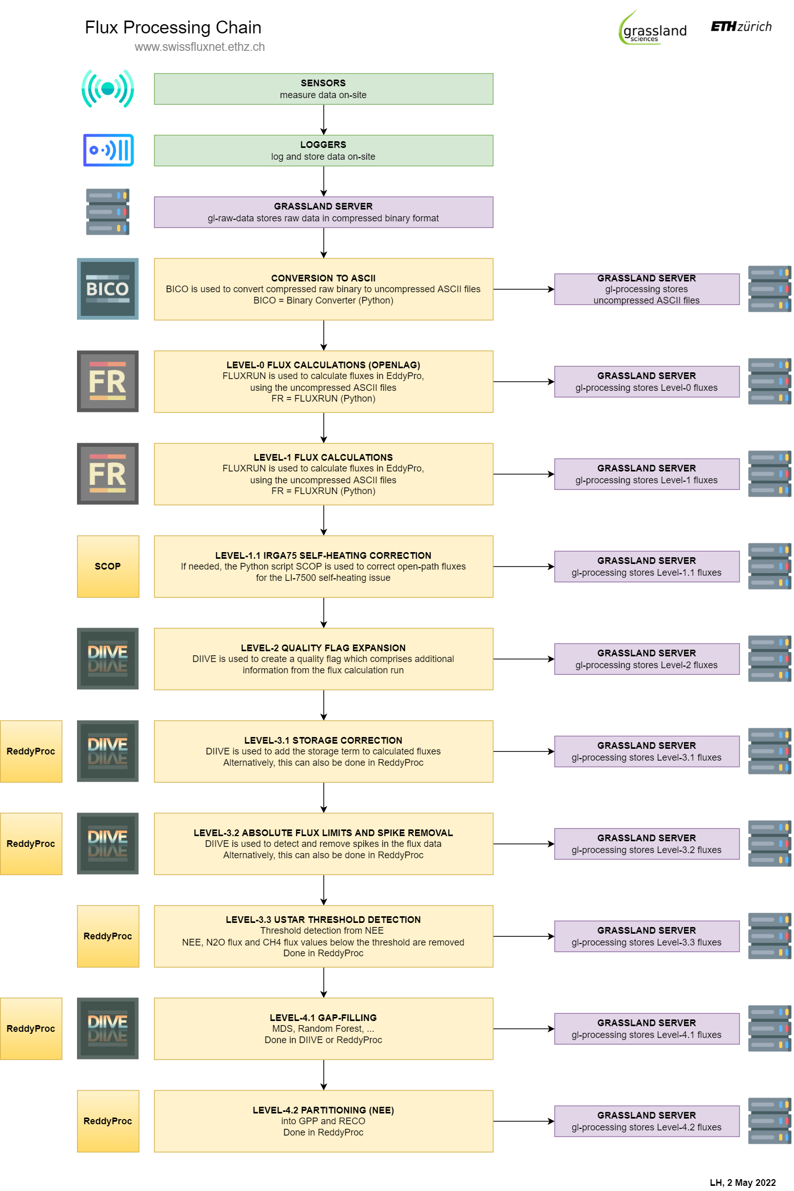
Step 1 | Raw Data Conversion
Conversion of eddy covariance raw data files from an irregular binary format to regular ASCII format
bico (Python script) converts compressed eddy covariance raw data binary files to uncompressed raw data files in ASCII format. After this conversion the files are human-readable and follow a consistent, regular format. Here, “regular” means that each data row has the same number of records. This regular format is needed for EddyPro flux calculations.
More info: EC Raw Data Binary Files
Required data: Compressed eddy covariance raw data binary files
Result: Uncrompressed eddy covariance raw data files in ASCII format
Software: bico (binary converter, Python script)
Done by: SRP (site-responsible persion, on-demand) and automatically (daily)
Step 2 | Level-0, Preliminary Flux Calculations With OPENLAG and Other Tests
Calculation of preliminary fluxes using preliminary EddyPro processing settings.
Basis for Level-1. Level-0 means “what you do is up to you”. No strict rules here. These fluxes are calculated throughout the year, on-demand by the SRPs (site-responsible persons) and automatically. Mainly used to check in on the site, e.g. if data are complete, if fluxes look plausible etc. Calculations are less strict than Level-1, e.g. the time window in which the lag time is searched is often much larger (10s+) without default time lag to check if the lag is still found as expected (OPENLAG). This information of lag times can then be used in Level-1 to narrow the time window to a more plausible range (typically 0-10s, or even lower for open-path IRGAs). Also, some settings might still not be final, e.g. some instrument settings (vertical separation of the IRGA) and to shorten calculation time the spectral correction might be set e.g. to Moncrieff et al. (1997), which is faster than e.g. Fratini et al. (2012) that is used for Level-1 calculations for some sites (IRGA72). On-demand Level-0 fluxes are currently calculated by the SRPs on their respective remote desktop server (RDSnx), the automatic Level-0 fluxes are calculated daily on a virtual machine running Windows.
Required data: ASCII raw data files from Step 1
Result: Preliminary fluxes
Software: fluxrun with EddyPro
Done by: SRP (on-demand, weekly), virtual machine (automatic, daily)
Step 3 | Level-1 Flux Calculations
Calculation of final fluxes using final EddyPro processing settings.
Basis for all following Levels. Strictly speaking, these calculations are independent from Level-0, but insights from Level-0 are used to improve Level-1 calculations, such as “Is the defined time window for lag search appropriate?”. These calculations make use of an additional input file that contains 6 meteo parameters (TA, PA, RH, SW_IN, LW_IN, PPFD_IN) that can be used to improve flux calculations. Note that after Level-1, calculated fluxes for (en)closed-path IRGAs (e.g., LI-7200) do not change anymore. However: For open-path systems (e.g., LI-7500), fluxes might need to be corrected for sensor self-heating (see Step 4).
Typical differences between Level-0 and Level-1 fluxes:
Level-1 fluxes have:
- often a narrower time window for lag search, e.g., 10 sec instead of 20 sec
- a different spectral correction, e.g. Fratini et al. (2012) for LI-7200 instead of Moncrieff et al. (1997)
- 6 meteo parameters as additional input
- additional output such as random uncertainty
- setup info such as sensor separation settings, i.e. the distance between SA and GA, is given as accurately as possible
- CO2 fluxes corrected for the IRGA75 self-heating (if needed)
Required data:
– ASCII raw data files from Step 1
– Final screened meteo data: TA, PA, RH, SW_IN, LW_IN, PPFD_IN (6 variables), variable abbreviations are described in the Variable Abbreviations
– OPENLAG results from Step 2, used to determine the size of the lag search window
Result: Level-1 fluxes that are used in the next processing steps
Software: fluxrun with EddyPro
Done by: PI/SRP
(Step 4 | Level-1.1: Self-Heating Correction for Open-Path IRGAs, if needed or if possible)
Correction for sensor self-heating for CO2 open-path fluxes from the LI-7500 (IRGA75), if needed or if possible.
Currently we are checking if water fluxes also need this correction.
Basis for Level-2. Note that after Level-1.1, calculated fluxes for open-path IRGAs (e.g., LI-7500) do not change anymore.
References: Burba et al. (2006) (PDF); Burba et al. (2008); Järvi et al. (2009); Kittler et al. (2017)
Important: The off-season uptake correction as implemented in EddyPro is never used in our EddyPro open-path flux calculations, since this implementation was developed for vertically mounted instruments and our IRGAs have an inclined sensor mounting. We also found that the EddyPro correction performed poorly when comparing corrected LI-7500 open-path fluxes to concurrent LI-7200 (en)closed-path fluxes.
Required data: Level-1 flux calculations from open-path IRGA that needs correction (e.g., LI-7500), and concurrently measured fluxes from a closed-path IRGA (e.g., LI-7200)
Result: Corrected fluxes following the approaches by Järvi et al. (2009) and Kittler et al. (2017) that can be used in the next processing steps
Software: Recent corrections for the forest sites CH-LAE and CH-DAV were done using the Python script SCOP.
Done by: PI/SRP
Step 5 | Level-2 Fluxes: Quality Flag Expansion
Extraction of additional information from the EddyPro full output file and creation of a new, expanded quality flag.
These are the same fluxes as in Level-1 (or Level-1.1), but an additional, extended quality flag is added to the output. QA/QC information from the Level-1 flux results are combined into a new quality flag QCF. For example, during this step, the “Signal Strength” of the IRGA72 is included in the extended quality flag QCF.
Important: USTAR filtering is NOT part of the Level-2 quality flag.
Required data: Level-1 fluxes
Result: An expanded flux quality control flag is added to the data:QCF (Quality Control Flag):
– QCF = 0 … best flux quality
– QCF = 1 … OK flux quality, can be used for budget calculations, but nighttime fluxes with QCF=1 should be rejected for budgets for most sites
– QCF = 2 … worst flux quality, it is recommended to always reject these fluxes
Software: DIIVE or custom scripts
Done by: PI/SRP
Step 6 | Level-3.1: Storage Correction
Storage term is added to Level-2 fluxes (CO2 flux, LE, H), calculated by addition: flux + the respective storage term
In this step, the storage terms are considered and NEE is calculated (important for forests; NEE = CO2 flux + storage term; the storage term is ideally calculated from profile measurements, but in case these are not available the EddyPro one-point storage term is used; normally negligible for grasslands).
Important: For CO2 fluxes it is easy to identify the storage-corrected flux because there is the defined abbreviation “NEE”: CO2 flux + CO2 flux storage term = NEE. For LE and H there is no default abbreviation to make clear that the respective flux was storage-corrected.
Required data: Level-1 fluxes
Result: Storage-corrected fluxes: NEE (CO2 flux + CO2 flux storage term), LE (LE + LE storage term), H (H + H storage term).
Software: DIIVE, ReddyProc, custom scripts
Done by: PI/SRP, FLUXNET
Step 7 | Level-3.2: Absolute Flux Limits and Outlier Removal
Application of absolute flux limits and removal of spikes in flux time series.
Basis for Level-3.3. Absolute flux limits are applied first, then outliers are removed, e.g., using rolling algorithms.
Important: Defining absolute flux limits can be tricky, but a good orientation to find meaningful limits is to look at only the highest quality fluxes (QCF = 0 from Level-2) and check their range. In most cases, these highes-quality fluxes show less scatter at the half-hourly scale and can therefore help in identifying a meaningful range for min/max limits.
Important: For many sites it makes sense to remove outliers separately for daytime and nighttime, i.e. it makes sense to run the algorithms separately on daytime and nighttime data, especially for NEE. Calculated nighttime fluxes can sometimes show unrealistic high uptake during dark conditions in the middle of the night. These high nighttime CO2 uptake fluxes can become problematic during gap-filling, because gaps are filled using available data. However, most of these nighttime CO2 uptake fluxes are removed during USTAR filtering.
Example: see flux post-processing, outlier removal during the creation of the PI dataset CH-DAV FP2022.5
Required data: Level-3.1 fluxes
Result: Despiked fluxes
Software: DIIVE, ReddyProc, custom scripts
Done by: PI/SRP, FLUXNET
Step 8 | Level-3.3: USTAR Filtering
Detection of the NEE USTAR threshold and removal of NEE fluxes where USTAR is below threshold.
Basis for Level-4.1.
USTAR threshold can be constant throughout all years or seasonal.
Currently, the NEE threshold is also applied to N2O and CH4 fluxes.
No threshold is applied to water fluxes (H2O, LE, ET) and the sensible heat flux (H), based on this reference:
The USTAR filtering is not applied to H and LE, because it has not been proved that when there are CO2 advective fluxes, these also impact energy fluxes, specifically due to the fact that when advection is in general large (nighttime), energy fluxes are small.
From: Pastorello, G. (2020). The FLUXNET2015 dataset and the ONEFlux processing pipeline for eddy covariance data. 27. https://doi.org/10.1038/s41597-020-0534-3
Required data: Level-3.2 fluxes
Result: Fluxes where time periods of low turbulence were removed.
Software: ReddyProc
Done by: PI/SRP, FLUXNET
Step 9 | Level-4.1: Gap-filling
Gaps in the flux time series are filled using MDS or other algorithms.
Basis for Level-4.2.
Gaps in NEE, water and energy fluxes are filled using the default method MDS (using SW_IN, TA and VPD) (Reichstein et al., 2005)
There is no generally agreed gap-filling method for N2O and CH4 fluxes, but random forest approaches work well (Maier et al., 2022).
Required data: Level-3.3 fluxes
Result: Gap-filled fluxes
Software: ReddyProc, DIIVE
Done by: PI/SRP, FLUXNET
Step 10 | Level-4.2: Partitioning (NEE)
Calculation of GPP and RECO from NEE.
Daytime partitioning method (Lasslop et al., 2010) is generally preferred. It is recommended to also include results from the nighttime partitioning method (Reichstein et al., 2005) and compare results to the daytime method.
Further reading regarding post-processing steps: Wutzler et al. (2018)
Water partitioning is not yet implemented by default in this step.
Required data: Level-4.1 fluxes
Result: GPP and RECO
Software: ReddyProc, DIIVE
Done by: PI/SRP, FLUXNET
Important Processing Chain Updates
- 16 May 2023: Added clarifications, reformatting.
- 15 Jun 2022: Extended description for Step 1.
- 2 May 2022: Each Level is now displayed as separate step. Updated flowchart.
- 17 May 2021: The application of absolute flux limits is now done in Level-3.2 (instead of Level-2). Therefore absolute flux limits are no longer included in the QCF quality flag.
- 12 May 2021: The correction of the IRGA75 self-heating issue is now Level-1.1 (instead of Level-3.1), the
QCFquality flag is not needed for the application of the correction. However, QCF is needed if the scaling factors for the correction need to be determined from parallel measurements, since these factors are calculated from highest quality data only.
Data Sharing
FLUXNET
For data sharing with FLUXNET see FLUXNET Requirements.
The flowchart has been designed using resources from Flaticon.com:
- server icon: https://www.flaticon.com/free-icon/server_3208726?term=server&page=1&position=8&page=1&position=8&related_id=3208726&origin=search
- logger: https://www.flaticon.com/free-icon/pc-tower_4179555?term=tower&page=1&position=6&page=1&position=6&related_id=4179555&origin=search
- sensor: https://www.flaticon.com/free-icon/sensor_2540167?term=sensor&page=1&position=17&page=1&position=17&related_id=2540167&origin=style
Last Updated on 18 Feb 2024 22:13