CH-LAE FP2021 (2004-2020)

Description

PI flux product FP2021 of CH-LAE ecosystem flux and meteo data over 17 years between 2004-2020.

This page gives an overview of the post-processing steps that were applied in generating the flux product FP2021.

This is the first PI dataset for CH-LAE. The dataset was released on 8 Jun 2021. The release-candidate-1 of the dataset was made available on 18 May 2021 and approved on 3 Jun 2021. The final FP2021 was presented and further discussed on 22 Jun 2021 (approx. 12 participants). Fluxes used in this dataset were uploaded to EFDC / FLUXNET on 9 Jun 2021 (for more info, see below in section Upload for FLUXNET / EFDC Data Sharing).

Important: The years 2004-2017 were corrected for open-path IRGA self-heating, refining the correction approach described by Kittler et al. (2017). For details, please see the section Note: Self-heating correction of open-path CO2 fluxes.

Links to references are given at the end of this page.

Before You Proceed

• Always look at the data with a critical eye.
• The dataset was created according to best current knowledge regarding processing and post-processing, but keep in mind that there are often multiple options to address different aspects in a long-term datasets, e.g. quality control, outlier removal, gap-filling, etc. I therefore tried to detail the central aspects of the applied post-processing on this page.
• The self-heating correction for the open-path fluxes is based on a time period of parallel measurements (IRGA75+IRGA72) 2016-2017. There is currently no way to validate this correction for old years (e.g., 2005). It is possible that open-path fluxes 10 years ago  needed a stronger or weaker self-heating correction than more recent years.
  More details about the self-heating correction are given below in the section Note: Self-heating correction of open-path CO2 fluxes, the code that was used can be found here:
  • Step 1, Calculating the scaling factors
  • Step 2, Applying the correction to open-path fluxes
• In case you do not agree with certain implementations in this dataset please feel free to contact me directly (holukas at ethz.ch), your input is very welcome and highly appreciated. If desired, there is also the possibility to get access to Level-1 fluxes (final calculated fluxes, without post-processing) to assemble your own long-term dataset.
• There are currently (June 2021) multiple studies in progress that look into the self-heating issue (and related issues) at multiple sites. One goal is to come up with a general approach to correct for this issue (unlikely) and for a method to detect for this issue at sites where parallel measurements (open-path+enclosed-path IRGAs) are not available (seems possible).
• You can link to this page directly using this QR Code:
  

Flux Products

• CH-LAE FP2021 (2004-2020)
  Release date: 8 Jun 2021
  Identifier: ID20210607205711
  Filename: CH-LAE_FP2021_2004-2020_ID20210607205711.csv

The release candidate release-candidate-1 (18 May 2021) was approved on 3 Jun 2021. There are differences between the release candidate and the final flux product:

• In the release-candidate-1, fluxes for 2018 were not corrected for the use of the Wrong Calibration Gas. This has been corrected in the final flux product FP2021.
• In the final flux product FP2021, in the IRGA72 data, the time periods between 19 May and 6 Jun 2018 (CO2 flux) and between 13 May and 6 Jun 2018 (LE) were set to missing data due to issues with the IRGA72 flowrate.

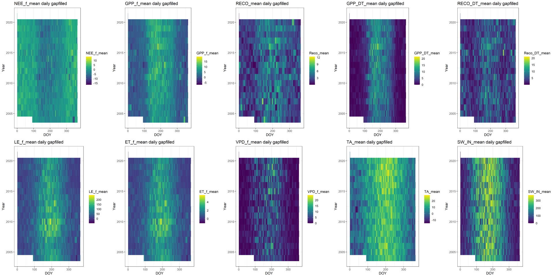
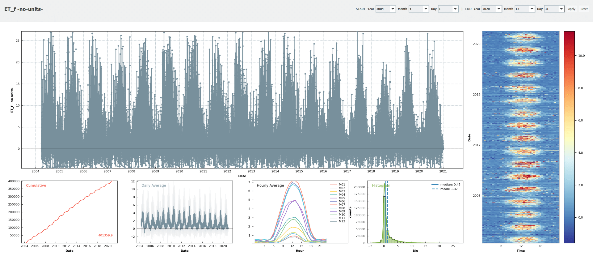
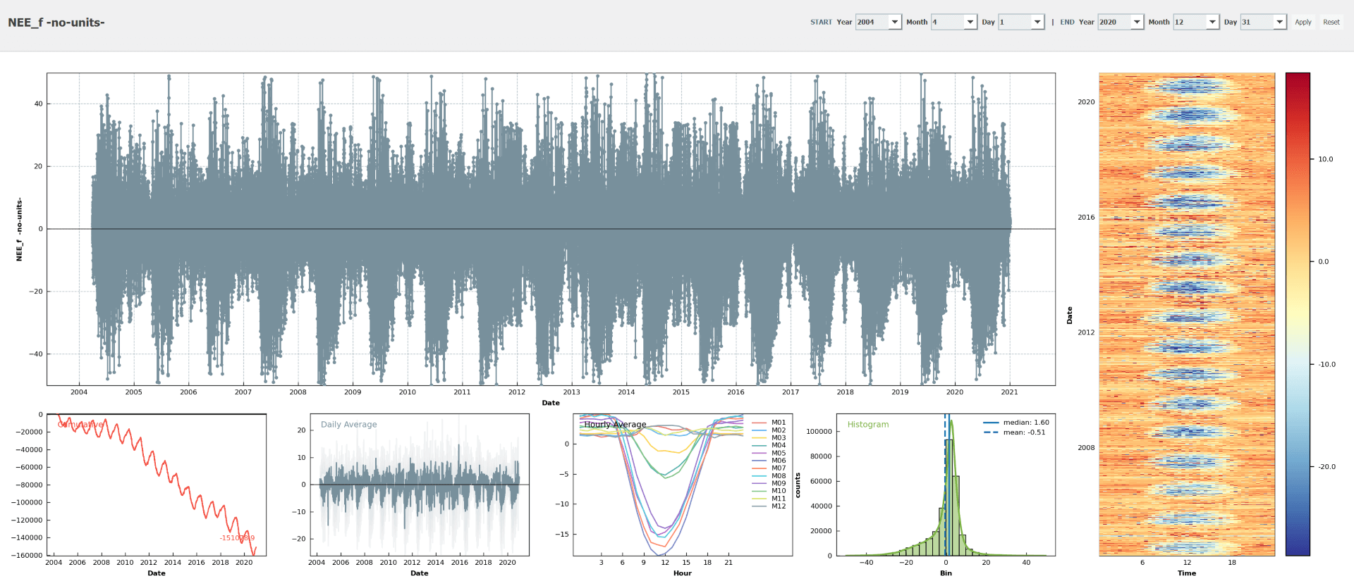
Plots

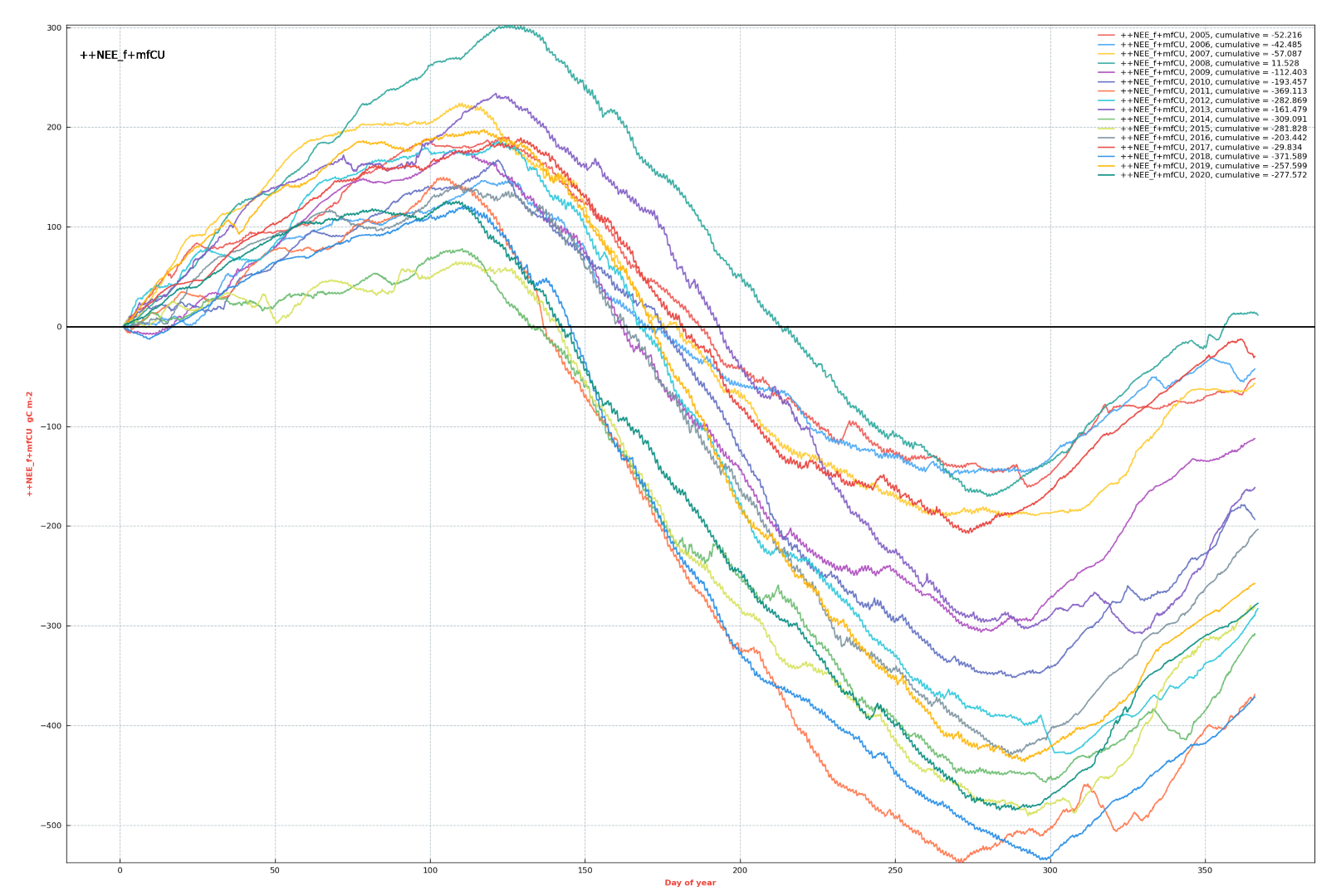
Key Stats

• Complete gap-filled years: 16 years (2005-2020)
• Time range: 1 Apr 2004 – 31 Dec 2020 (17 years, 6118 days)
• Available measured values: after all quality checks, outlier removal and ustar threshold application
  • NEE_f: 42.6% measured / 57.4% gap-filled
  • LE_f and ET_f: 63.9% measured / 36.1% gap-filled
• Available data after gap-filling: 293712 half-hourly fluxes
• Ustar threshold: 0.3, constant through all years (for carbon fluxes)
• Best estimate cumulative carbon uptake (2005-2020, 16 years): 2.99 kg C m^-2 (NEE_f), avg. 0.187 kg C m^-2 yr^-1
• Carbon source / sink behavior: The site is a sink for CO2 in 15 of 16 complete years (NEE_f)

Dataset Contents

• List of dataset variables:

  TIMESTAMP,E_0,ET_f,FP_alpha,FP_alpha_sd,FP_beta,FP_beta_sd,FP_dRecPar,FP_E0,FP_E0_sd,FP_errorcode,FP_GPP2000,FP_k,FP_k_sd,FP_NEEnight,FP_qc,FP_RRef,FP_RRef_Night,FP_RRef_sd,FP_Temp,FP_VARday,FP_VARnight,GPP_DT,GPP_DT_SD,GPP_f,GPP_fqc,LE_f,LE_fall,LE_fall_qc,LE_fmeth,LE_fnum,LE_fqc,LE_fsd,LE_fwin,LE_orig,NEE_f,NEE_fall,NEE_fall_qc,NEE_fmeth,NEE_fnum,NEE_fqc,NEE_fsd,NEE_fwin,NEE_orig,NEW_FP_Temp,NEW_FP_VPD,PotRad,PotRad_NEW,QCF_H_QC01_IRGA7572,QCF_LE_QC01_IRGA7572,QCF_NEE_QC01_IRGA7572,R_ref,Reco,Reco_DT,Reco_DT_SD,Rg_f,Rg_fall,Rg_fall_qc,Rg_fmeth,Rg_fnum,Rg_fqc,Rg_fsd,Rg_fwin,Rg_orig,Tair_f,Tair_fall,Tair_fall_qc,Tair_fmeth,Tair_fnum,Tair_fqc,Tair_fsd,Tair_fwin,Tair_orig,Unnamed: 0,VPD_f,VPD_fall,VPD_fall_qc,VPD_fmeth,VPD_fnum,VPD_fqc,VPD_fsd,VPD_fwin,VPD_orig,_TIMESTAMP_END

• For an explanation of variables in the output file, please see ReddyProc Data Output Format and List of Variables
• Missing values: -9999

Dataset Production

For info about the flux processing chain and flux levels see:: Flux Processing Chain

Software

• EddyPro v6 and v7 for flux calculations (links to details of Level-1 fluxes are given below for each year)
• BICO for the conversion of binary raw data files to ASCII (2016, 2017, 2018, 2020)
• FLUXRUN for the flux calculation using EddyPro (2016, 2017, 2018, 2020)
• Various versions of FCT (flux calculation using EddyPro) and FQC (flux quality control) were used for earlier years and 2019, details are given in the section Used Flux Versions below
• The self-heating correction of IRGA75 fluxes was done in Juypter Notebooks, see section below: Note: Self-heating correction of open-path CO2 fluxes
• DIIVE v0.19.0-alpha for file merging, quality control, storage correction, outlier removal, application of the constant ustar threshold
• ReddyProc v1.2.2 for MDS gap-filliing and partitioning, in R Studio v1.3.959

Setup

• Setup since 2004

General Steps

Level-1 / Collection: The most recent Level-1 fluxes for all IRGAs were collected.

Step 1: Separate for each IRGA dataset

1. Level-1 / Corrections before merging (IRGA75 in 2013):
   • In the IRGA75 Level-1 fluxes, the timestamp of flux variables between 6 Jul and 12 Jul 2013 (6 days) was shifted by approx. 14.5 hours
     • Affected time range: between 2013-07-06 15:45 and 2013-07-12 23:45.
     • For example, data at timestamp 2013-07-06 15:45 is really 2013-07-06 08:15.
     • Level-1 data were shifted accordingly. Then, the transition day 2013-07-12 was set to missing.
2. Level-1 / Merging: All available Level-1 fluxes were merged for each IRGA separately. This resulted in two separate IRGA datasets: one for IRGA75 (2004-2017, 2019_3) and one for IRGA72 (2016-2020).
3. Level-1.1 / Correction for IRGA75 self-heating: (For more details see note below) For the IRGA75 dataset (2004-2017+2019_3), CO2 fluxes were corrected for the IRGA75 self-heating issue, following the approach described in Kittler et al. (2017). A direct comparison of IRGA75 / IRGA72 parallel measurements (2016-2017) revealed that the CO2 flux measured by the IRGA75 strongly overestimates CO2 uptake rates and underestimates CO2 emission in comparison to the IRGA72. This effect was strong throughout the year and not restricted to the cold season. It is possible that a similar effect is also present for water fluxes but this needs further investigation. A quick comparison of the parallel measurements seemed to indicate that IRGA75 water fluxes show approximately 10% higher water release between 2016 and 2017 (time period of parallel measurements, approx. 20 months) than IRGA72 water fluxes.
   The self-heating correction needs the meteo data air temperature (TA) and shortwave-incoming radiation (SW_IN) as input variables, in combination with flux output generated during Level-1 calculations. PPFD is also used, but only as an auxiliary variable to help dividing data into daytime and nighttime data.
   • For SW_IN (2004-2019), SW_IN_F from FLUXNET (2004-2018) was used because it had data for the first years (2004-2005) included. It also had the negative values removed, which was not the case in our screened meteo files. Data for 2019 were added from our respective meteo files.
   • For TA (2004-2019), gaps in the time series were gap-filled using TA_F from FLUXNET (2004-2018) because it had data for 2004 included. Data for 2019 were added from our respective meteo files.
   • For PPFD (Sep 2004-2019) data from our meteo files were used.
4. Level-2 / Quality Control: For each IRGA dataset separately, extended quality flags were created, based on the merged dataset of the respective IRGA. The quality flag for the fluxes is called QCF and was created for: CO2 flux, LE and H. Bad flux values (QCF = 2) were removed from the dataset. The selection of quality criterions is based on Sabbatini et al. (2018). No absolute flux limits were applied in this step (this is done in Level-3.2).
   Additional QC: In the IRGA72 dataset, the time periods between 19 May and 6 Jun 2018 (CO2 flux) and between 13 May and 6 Jun 2018 (LE) were set to missing data due to issues with the IRGA72 flowrate.
5. Level-3.1 / Storage correction: For each IRGA dataset separately, the respective storage terms were added to CO2 flux, LE and H. This step yields NEE for the CO2 flux.

After Level-3.1 was generated for each IRGA dataset, a subset containing only NEE, LE, H, QCFs and ustar was created for each IRGA. These two datasets are merged in the next step.

Step 2: For the combined dataset IRGA75 + IRGA72

1. Level-3.1 / Merging of IRGA75 and IRGA72 subset datasets: Data from both datasets were merged into one file. Data from the IRGA75 dataset have the suffix _IRGA75, data from the IRGA72 have the suffix _IRGA72. Fluxes (NEE, LE, H) from the two IRGAs were then collected in one single column, marked by the suffix _IRGA7572. For the merging, the IRGA72 fluxes were used as the starting dataset. Then, the IRGA75 fluxes were added, filling data gaps in the time series with IRGA75 values. In the time period where IRGA75 and IRGA72 fluxes overlap (2016-2017), priority was given to IRGA72 fluxes, but IRGA75 fluxes were used to fill gaps in the IRGA72 fluxes whenever possible. This was done not only for the fluxes, but also for the QCF data. This way all data points should have their respective correct data flag, even though there is this mixing of IRGAs with sometimes different QCF criteria.
2. Level-3.2 / Outlier removal and application of absolute flux limits:For the combined IRGA datasets:
   • Step 1: Application of absolute flux limits:
     • NEE: values outside a physically plausible range of ±50 µmol CO₂ m^-2 s^-1 were considered outliers
     • LE: range between -200 and +1200 W m^-2
     • H: range between -200 and +1000 W m-2
     • Note that this step was done before the application of the Hampel filter in the next step, so that the Hampel filter has a similar data basis (data range) for all years. The IRGA75 fluxes show generally considerably more noise than IRGA72 fluxes.
   • Step2: NEE were despiked using a Hampel filter using the median absolute deviation (MAD) in a running time window of 432 records (9 days). The limit above which a NEE data point was defined as an outlier was set at 5 sigmas (NEE). The same filter was used for LE, with the exception that 20 sigmas (weak outlier removal) were used for the outlier limit. Weak outlier removal was done for H with a running median filter (not Hampel) with a SD range multiplier of 6 and a running time window of 432 records (9 days). The filters were applied multiple times until all outliers were removed from the dataset.
   • Step 3: Trimming of potential non-biotic NEE fluxes during the cold season:
     High positive and negative fluxes during the cold season between October and February have been interpreted as non-biotic fluxes that are possible related to weathering or dissolving processes of calcareous soil substances (Etzold et al., 2011). These fluxes were kept in the dataset, but highest and lowest fluxes were removed following a trimmed mean approach. First, all data between October and February for all years (2004-2020) were pooled. Then, fluxes below the 0.5th percentile and above the 99.5th percentile were removed.
     

     CH-LAE (2004-2020): Effect of trimming NEE during the cold season to the 0.5 – 99.5 percentile range between October and February.

3. Level-3.3 / ustar Threshold: A constant threshold of 0.3 m s^-1 was used. All NEE values where ustar was below this threshold were removed in Flux Level-3. The threshold is in accordance with previous studies (Etzold et al., 2011; Paul-Limoges et al., 2017) and with the median from FLUXNET ustar analyses using data from 2005-2018 (CUT50, the median from 200 bootstrap runs using two different methods). The threshold was not applied to energy fluxes LE and H.
4. Level-4.1 / Gap-filling:
   • Done using ReddyProc
   • Fluxes of quality QCF = 0 and QCF = 1 were gap-filled.
   • The following variables were used from the FLUXNET Drought 2018 dataset (2004-2018), data for the years 2019 and 2020 were then added from our meteo files :
     • SW_IN_F was used for gap-filling because it had data for the first years (2004-2005) included. It also had the negative values removed, which was not the case in our screened meteo files.
     • Gaps in the TA time series were gap-filled using TA_F from FLUXNET because it had data for 2004 included.
     • RH because it was already corrected for values larger than 100%.
     • VPD_F because it comprised data for 2004. VPD was also calculated during post-processing from gap-filled TA and not-gap-filled RH, which was then combined with the FLUXNET VPD to yield the complete time series 2004-2020. Remaining gaps (in 2019 and 2020) were then gap-filled using MDS.
     • Remaining issues with the meteo data (e.g. values below zero for SW_IN in 2019 and 2020) were then removed in ReddyProc.
     • For a description of the used FLUXNET meteo variables see here: FLUXNET FULLSET Data Product
5. Level-4.2 / Partitioning (NEE):
   • Done using ReddyProc
   • Two different versions of GPP and RECO were calculated:
     • Nighttime-based partitioning after Reichstein et al. (2005), using sMRFluxPartition
     • Daytime-based partitioning after Lasslop et. al (2010), using sGLFluxPartition

Note: Self-heating correction of open-path CO2 fluxes

This section gives more details about Level-1.1.

CO2 fluxes from the open-path IRGA75 (LI-7500) are affected by the self-heating of the instrument, which leads to an overestimation of CO2 uptake / underestimation of CO2 emissions.

The open-path IRGA at CH-LAE was mounted in an inclined position. The self-heating correction in EddyPro (Burba et. al., 2008) can therefore not be applied since it was developed for vertically mounted sensors. Here we describe the approach how open-path fluxes at CH-LAE (2004-2017) were corrected, following Kittler et al. (2017) and Järvi et al. (2009).

An optimized scaling factor was calculated based on the time period of parallel measurements (2016-2017). The scaling factor was then used to correct all open-path LI-7500 years (2004-2017+2019_3) for self-heating.

Code

• Jupyter notebooks with the code can be found here:
  • Step 1, Calculating the scaling factors
  • Step 2, Applying the correction to open-path fluxes

Summary

For CH-LAE, we had a time period of approx. 20 months of parallel IRGA measurements available, during which the CO2 flux was calculated for both the open-path IRGA75 and the enclosed-path IRGA72. A comparison of the fluxes of the two instruments showed a significant difference in calculated CO2 fluxes. For CH-LAE, this difference can be corrected following the approach described in Kittler et al. (2017), based on Burba et al. (2006).

• Open-path fluxes not corrected for self-heating overestimated the measured high-quality CO2 uptake over 20 months (2016-2017) by +41%.
• After the correction, this difference between the two instruments was reduced to +5%.
• The self-heating effect was strong throughout the year and not restricted to the cold season:
  • Between March and May (1425 half-hours):
    • uptake overestimated by +69%, after correction +4%
  • Between June and August (3142 half-hours):
    • uptake overestimated by +19%, after correction +2%
  • Between September and November (2049 half-hours):
    • uptake overestimated by +73%, after correction +12%
  • Between December and February (881 half-hours):
    • emission from open-path not corrected for self-heating: 2 gC m-2
    • from enclosed path (“true” flux): 50 gC m-2
    • from open-path corrected for self-heating: 38 gC m-2

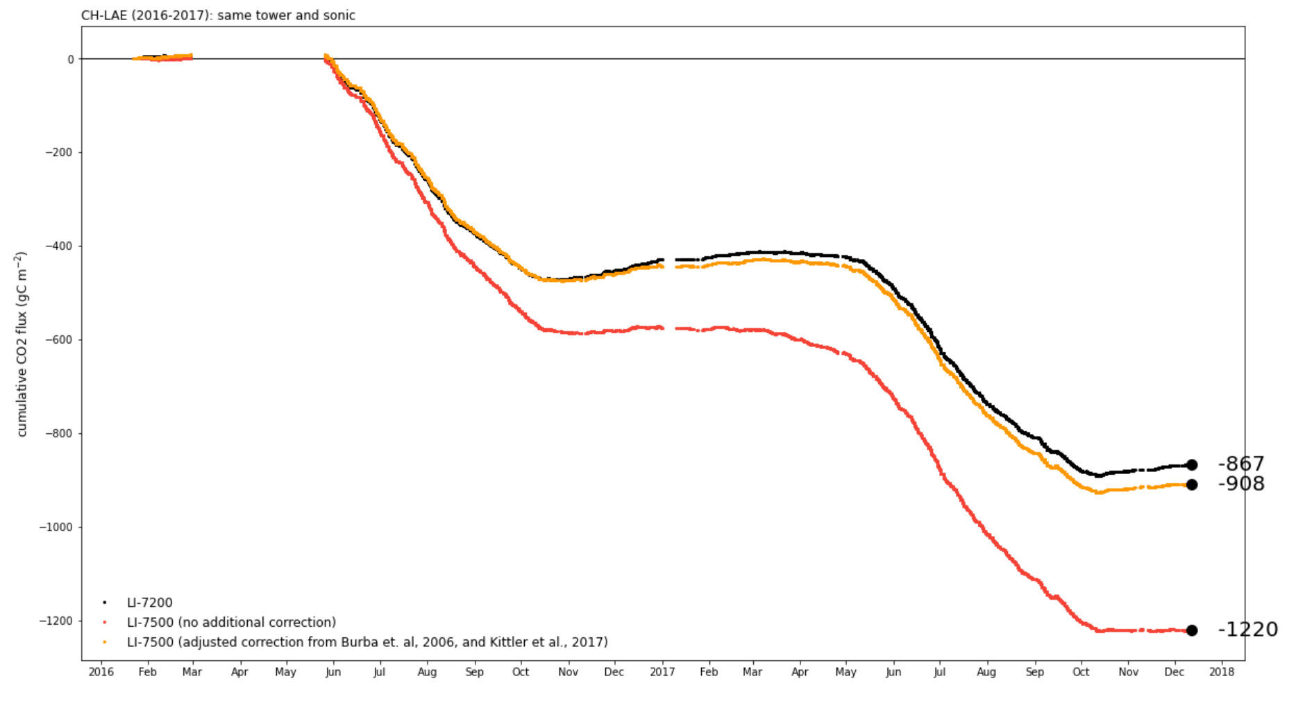
Figure A Cumulative CO2 fluxes (gC m-2)

Figure A shows the cumulative CO2 flux (gC m-2) calculated from the open-path IRGA (LI-7500) and the enclosed-path IRGA (LI-7200) during the time period of parallel measurements between 2016 and 2017. The red line shows LI-7500 fluxes after full processing (including WPL correction), but without self-heating correction. The orange line shows the same LI-7500 fluxes, but corrected for the self-heating using an approach based on Kittler et al. (2017). The black line shows concurrent fluxes measured by an enclosed-path analyzer which is not affected by the self-heating and was therefore considered the “true” flux. Figure A is based on high-quality fluxes (quality flag = 0, best).

The correction was done by adding a scaled flux correction term to the calculated open-path fluxes, simplified:

corrected flux = calculated flux + scaling factor * flux correction term

The calculated flux refers to the LI-7500 flux after full processing (including WPL correction and quality control), but without self-heating correction.

Flux correction term (unscaled)

First, the (unscaled) flux correction term was calculated for all data rows following eq.(5) in Kittler et al. (2017), using the variables:

• instrument surface temperature (calculated according to eq.(8) in Järvi et al., 2009; using ambient air temperature)
• ambient air temperature
• ambient CO2 density
• partial density of H2O
• partial density of dry air (calculated from air density, water vapor density, molar mass of dry air and molar mass of water vapor)
• molar mass ratio of dry air to water vapor (constant 1.6077)
• aerodynamic resistance (calculated from horizontal wind speed and ustar)

Figure B Diel cycles (2004-2020) per hour and month of the (unscaled) flux correction term, calculated according to eq.(8) in Järvi et al. (2009).

Scaling factor

The scaling factor determines how much of the (unscaled) flux correction term is added to the calculated flux that needs correction. For CH-LAE, we found a nearly linear relationship between the scaling factor ξ and ustar (friction velocity). Therefore, ξ was optimized in 20 classes of ustar, separate for daytime and nighttime, using a least squares method (bootstrap with replacement) to find the best agreement between LI-7500 and LI-7200 fluxes between 2016 and 2017 (time period of parallel measurements) (Figure C).

Figure C The scaling factor in 20 classes of ustar, separate for daytime and nighttime, calculated from the time period of parallel measurements (2016-2017).

Figure D Diel cycles (2004-2017+2019_3) of the scaling factor, per hour and month, from the full 14-year LI-7500 dataset.

Scaled flux correction term

The scaled flux correction term is calculated by multiplying the (unscaled) flux correction term by the scaling factor, done for each data row in the LI-7500 dataset (2004-2017+2019_3). The scaled flux correction term was then added to the calculated CO2 fluxes that need correction (2004-2017+2019_3).

Figure E Diel cycles (2004-2017+2019_3, LI-7500 dataset) per hour and month of the scaled flux correction term, calculated by multiplying the (unscaled) flux correction term by the scaling factor.

Example correction in EddyPro

Here is an example of how the correction following Burba et al. (2008) and using EddyPro performs in comparison to the selected correction method. The plot was generated during a different run than the plots shown above, which is why the numbers are slightly different.

Figure F shows the cumulative CO2 flux (gC m-2) calculated from the open-path IRGA (LI-7500) and the enclosed-path IRGA (LI-7200) during the time period of parallel measurements between 2016 and 2017.

• The red line shows LI-7500 fluxes after full processing (including WPL correction), but without self-heating correction.
• The orange line and the blue line show the same LI-7500 fluxes, but corrected for the self-heating (1) using an approach based on Kittler et al. (2017) (orange line) and (2) using the approach for vertically mounted sensors from Burba et al. (2008) as implemented in EddyPro (blue line).
• The black line shows concurrent fluxes measured by an enclosed-path analyzer which is not affected by the self-heating and was therefore considered the “true” flux.

Figure F is based on high-quality fluxes (quality flag = 0, best).

Figure F Comparison of the the selected correction method and results from EddyPro (cumulative NEE in gC m-2 between 2016 and 2017). The blue line shows the correction as it is currently implemented in EddyPro (for vertically mounted sensors).

Used Flux Versions

2004-2017 + 2019_3: HS50-IRGA75

• 2004 HS50-IRGA75_FF-201606 / Level-1_ID2016-06-11T172228
• 2005 HS50-IRGA75_FF-201606 / Level-1_ID2016-06-13T160226
• 2006 HS50-IRGA75_FF-201606 / Level-1_ID2016-06-11T172802
• 2007 HS50-IRGA75_FF-201606 / Level-1_ID2016-06-11T173003
• 2008 HS50-IRGA75_FF-201606 / Level-1_ID2016-06-13T134346
• 2009 HS50-IRGA75_FF-201606 / Level-1_ID2016-06-10T163717
• 2010 HS50-IRGA75_FF-201606 / Level-1_ID2016-06-10T163705
• 2011 HS50-IRGA75_FF-201606 / Level-1_ID2016-06-10T163655
• 2012 HS50-IRGA75_FF-201606 / Level-1_ID2016-06-11T172208
• 2013 HS50-IRGA75_FF-201606 / Level-1_ID2016-06-10T163630
• 2014 HS50-IRGA75_FF-201606 / Level-1_ID2016-06-10T163622
• 2015 HS50-IRGA75_FF-201606 / Level-1_ID2016-06-10T163549
• 2016 HS50-IRGA72-IRGA75_FF-202101 / Level-1_DIIVE-20210606-105901 (IRGA75)
• 2017 HS50-IRGA72-IRGA75_FF-202101 / Level-1_DIIVE-20210606-105902 (IRGA75)
• 2019 HS50-IRGA75-IRGA72_FF-202101 / Level-1_DIIVE-20210607-093449 based on flux calcs in FF-202006 / Level-1_ID2020-06-27T001433 (short period 2019_3 for IRGA75), these are the same fluxes but corrected for self-heating

2016-2020: HS50-IRGA72

• 2016 HS50-IRGA75_FF-202101 / Level-1_DIIVE-20210606-105901 (IRGA72)
• 2017 HS50-IRGA75_FF-202101 / Level-1_DIIVE-20210606-105902 (IRGA72)
• 2018 HS50-IRGA72_FF-202101 / Level-1_DIIVE-20210607-093447
• 2019 HS50-IRGA75-IRGA72_FF-202101 / Level-1_DIIVE-20210607-093449 based on flux calcs in Level-1_ID2020-06-27T001433 (time periods 2019_1-2-4 for IRGA72), same fluxes as in FF-202006 / Level-1_DIIVE-20210607-093449
• 2020 HS50-IRGA72_FF-202101 / Level-1_FR-20210419-120722

Upload for FLUXNET / EFDC Data Sharing

IRGA75 Level-1.1 fluxes (corrected for self-heating, 2004-2017) were combined with IRGA72 Level-1 fluxes (2016-2020).

IRGA75 Level-1.1 fluxes (2004-2017, corrected for self-heating)

• Quality check: Rejected CO2 and LE flux values where AGC > 90 (bad quality) or AGC < 50 (range of AGC is typically between 50 and 100, with the exception that in 2019 an AGC of 43.75 = best quality)
• Preparation for merging with IRGA72 data:
  • This is necessary so that records from the different IRGAs match after merging data from the two IRGAs in the years of parallel measurements (2016-2017)
  • For CO2, keep storage, mole fraction and SSITC flag where we have CO2 flux available
  • For LE, keep storage, H2O mole fraction and SSITC flag where we have LE flux available
  • For H, keep storage and SSITC flag where we have H flux available
• Rename variables to FLUXNET Requirements

IRGA72 Level-1 fluxes (2016-2020)

• Quality check:
  • Rejected CO2 and LE flux values where signal strength < 50 (bad quality)
  • The time periods between 19 May and 6 Jun 2018 (CO2 flux) and between 13 May and 6 Jun 2018 (LE) were set to missing data due to issues with the IRGA72 flowrate.
• Preparation for merging with IRGA72 data:
  • This is necessary so that records from the different IRGAs match after merging data from the two IRGAs in the years of parallel measurements (2016-2017)
  • For CO2, keep storage, mole fraction and SSITC flag where we have CO2 flux available
  • For LE, keep storage, H2O mole fraction and SSITC flag where we have LE flux available
  • For H, keep storage and SSITC flag where we have H flux available
  • Rename variables to FLUXNET Requirements

Merging IRGA72+IRGA75

• Both datasets were combined into one merged dataset
• IRGA72 fluxes were prioritized in overlapping years (2016-2017), gaps were filled with IRGA75 fluxes (if available for the IRGA72 gap)
• Exported each year to separate file with yearly range (2004-2020)
• Uploaded yearly files to EFDC / FLUXNET (9 Jun 2021)

Known Issues

• The self-heating of the IRGA75 is potentially also affecting water fluxes. From measured data it seems that IRGA75 fluxes show approx. 10% more water release than IRGA72 fluxes (2016-2017 parallel measurements).

References

Last Updated on 16 Feb 2024 00:10

References

- Burba, G. G., Anderson, D. J., Xu, L., & McDermitt, D. K. (2006). Correcting apparent off-season CO2 uptake due to surface heating of an open path gas analyzer: Progress report of an ongoing study. 13.
-
Burba, G. G., McDERMITT, D. K., Grelle, A., Anderson, D. J., & Xu, L. (2008). Addressing the influence of instrument surface heat exchange on the measurements of CO 2 flux from open-path gas analyzers. Global Change Biology, 14(8), 1854–1876. https://doi.org/10.1111/j.1365-2486.2008.01606.x
- Etzold, S., Ruehr, N. K., Zweifel, R., Dobbertin, M., Zingg, A., Pluess, P., Häsler, R., Eugster, W., & Buchmann, N. (2011). The Carbon Balance of Two Contrasting Mountain Forest Ecosystems in Switzerland: Similar Annual Trends, but Seasonal Differences. Ecosystems, 14(8), 1289–1309. https://doi.org/10.1007/s10021-011-9481-3
- Järvi, L., Mammarella, I., Eugster, W., Ibrom, A., Siivola, E., Dellwik, E., Keronen, P., Burba, G., & Vesala, T. (2009). Comparison of net CO2 fluxes measured with open- and closed-path infrared gas analyzers in an urban complex environment. 14, 16.
- Kittler, F., Eugster, W., Foken, T., Heimann, M., Kolle, O., & Göckede, M. (2017). High-quality eddy-covariance CO 2 budgets under cold climate conditions: Arctic Eddy-Covariance CO 2 Budgets. Journal of Geophysical Research: Biogeosciences, 122(8), 2064–2084. https://doi.org/10.1002/2017JG003830
Lasslop, G., Reichstein, M., Papale, D., Richardson, A. D., Arneth, A., Barr, A., Stoy, P., & Wohlfahrt, G. (2010). Separation of net ecosystem exchange into assimilation and respiration using a light response curve approach: Critical issues and global evaluation: SEPARATION OF NEE INTO GPP AND RECO. Global Change Biology, 16(1), 187–208. https://doi.org/10.1111/j.1365-2486.2009.02041.x
- Paul-Limoges, E., Wolf, S., Eugster, W., Hörtnagl, L., & Buchmann, N. (2017). Below-canopy contributions to ecosystem CO 2 fluxes in a temperate mixed forest in Switzerland. Agricultural and Forest Meteorology, 247, 582–596. https://doi.org/10.1016/j.agrformet.2017.08.011
Sabbatini, S., Mammarella, I., Arriga, N., Fratini, G., Graf, A., Hörtnagl, L., Ibrom, A., Longdoz, B., Mauder, M., Merbold, L., Metzger, S., Montagnani, L., Pitacco, A., Rebmann, C., Sedlák, P., Šigut, L., Vitale, D., & Papale, D. (2018). Eddy covariance raw data processing for CO2 and energy fluxes calculation at ICOS ecosystem stations. International Agrophysics, 32(4), 495–515. https://doi.org/10.1515/intag-2017-0043
Last Updated on 5 Oct 2024 13:15