CH-AWS FP2022 (2015-2021)
PI dataset of CH-AWS fluxes 2015-2021.
STATUS: Released.
Contents
Flux Products
For an explanation of variables in output files, please see Variable Abbreviations and ReddyProc Data Output Format
FP2022.1
- Date: 8 Feb 2022
- Identifier:
ID20220202233037 - File:
CH-AWS_FP2022.1_2015-2021_ID20220202233037_30MIN.csv - Description: Initial release using a variable USTAR threshold for all years, MDS gap-filling and partitioning done in ReddyProc
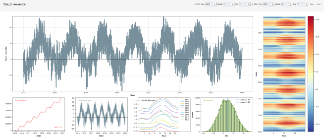
- Included variables: NEE, GPP, Reco, TA, SW_IN, VPD and auxiliary output
- Recommended flux variables:
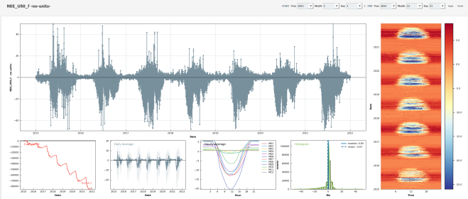
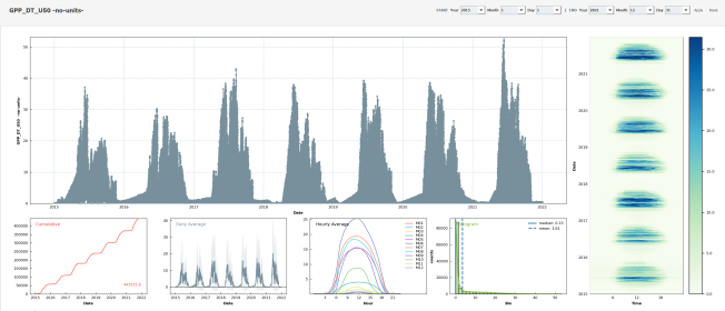
- gap-filled: NEE_U50_f, GPP_DT_U50, Reco_DT_U50, LE_f, ET_f
- It is recommended to use GPP and Reco from the daytime partitioning method (_DT), because daytime fluxes are generally more reliable across years. However, partitioned fluxes from the nighttime method are also included in this dataset.
- measured only (highest quality): NEE_CUT_QCF0, LE_QC0
- Release candidates:
- None
Plots
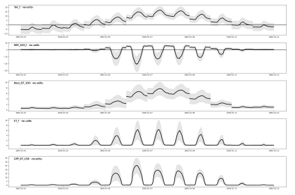
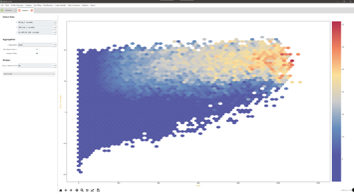
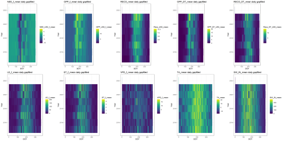
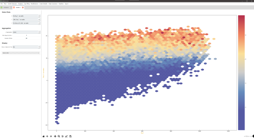
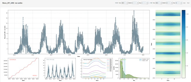
Description
- Ecosystem fluxes over 7 years from two different IRGAs and sonic anemometers
- This is the first version of the CH-AWS PI dataset.
Key Stats
- Best estimate cumulative carbon uptake (2015-2021): 1.8 kg C m-2 (
NEE_U50_f), avg. 254 g C m-2 yr-1 - Available directly measured, highest-quality fluxes:
- directly measured fluxes with quality flag
QCF= 0 (no gap-filling) NEE_U50_QCF0: 37680 half-hours (30.7% of potential values) [1], [2], [3]LE_QCF0: 32938 half-hours (26.8% of potential values) [1], [3]
- directly measured fluxes with quality flag
- Data basis for budget calculations:
NEE_U50_f: 46.5% measured / 53.5% gap-filled [1], [2], [4]LE_fandET_f: 45.7% measured / 54.3% gap-filled [1], [4]
[1] … after all quality checks, including outlier removal
[2] … after USTAR threshold application
[3] … QCF = 0 (daytime and nighttime)
[4] … measured data include quality flag QCF = 0 and QCF = 1 (OK quality) for daytime data, and QCF = 0 for nighttime data
Dataset Production
- For info about the flux processing chain and flux levels see: Flux Processing Chain
- Google Sheet that was used to document processing progress: CH-AWS / FP2022 (2015-2021)
Software
- bico v1.2.1 for the conversion of binary raw data files to ASCII
- fluxrun v1.0.3 for the flux calculation using EddyPro v7.0.8
- diive v0.21.0 (legacy version) for file merging, quality control, storage correction, outlier removal
- ReddyProc v1.2.2 for USTAR threshold detection, MDS gap-filliing and partitioning, in R Studio v1.3.959
Processing Steps
For an overview of the general processing chain see here: Flux Processing Chain
Steps to create a flux dataset comprising CO2 flux (NEE), LE and H. Note that H2O flux and ET are not prepared, only LE is used from the water fluxes. ET is later calculated (converted from LE) in ReddyProc.
Level-1 / Flux calculations 2015-2021
- for IRGA75 (2015) and IRGA72 (2015-2021) fluxes
Source Data
- Using data from the Adaptive Setup since 2015 (2015-2021) and Mobile Setup 2006-2016 (2015), for an overview of raw data see here: EC Raw Binary Format (CH-AWS)
Flux Data (Level-1)
2015-2021: HS50-IRGA72
- 2021 Level-1_FR-20220127-164245
- 2020 Level-1_FR-20220111-201927
- 2019 Level-1_XXX: FR-20220126-164653 + FR-20220111-202059
- 2018 Level-1_FR-20220111-202307
- 2017 Level-1_FR-20220126-133051
- 2016 Level-1_FR-20220111-202533
- 2015 Level-1_FR-20220126-131843
2015: R2-IRGA75
- 2015 Level-1_FR-20220126-170707
Meteo Data
TA (Tair), SW_IN (Rg), RH, VPD meteo data (2021) were merged with meteo data from the FLUXNET Warm Winter 2020 dataset (2015-2020)
Last Updated on 5 Oct 2024 13:15