Defining The Correct Lag-time
For more information about Flux Levels please see here.
In some cases, e.g. when using a new instrument that was never used before, it is not known in which team window the maximum covariance between tubulent wind and the scalar of interest (CO2, H2O, etc…) should be searched.Therefore, it is recommended to first search for lag times in a relatively large time window (“open-lag run”) and check the histogram of found lag times and whether any peak in the distribution can be seen. Then – for the final flux calculations – search the lag again in a smaller time window. The smaller time window is defined according to the histogram of found lag times from the open-lag run. The peak of the histogram can be used as the nominal / default lag time in EddyPro (used when no clear maximum covariance was found).
Here is an example for determining the correct lag time using sonic wind data and N2O mixing ratios from an LGR instrument for the site CH-OE2.
- Run EddyPro and let it search the lag time of interest in a relatively large time window, e.g. here we search the maximum covariance between tubulent wind and N2O mixing ratio between 0-10s.
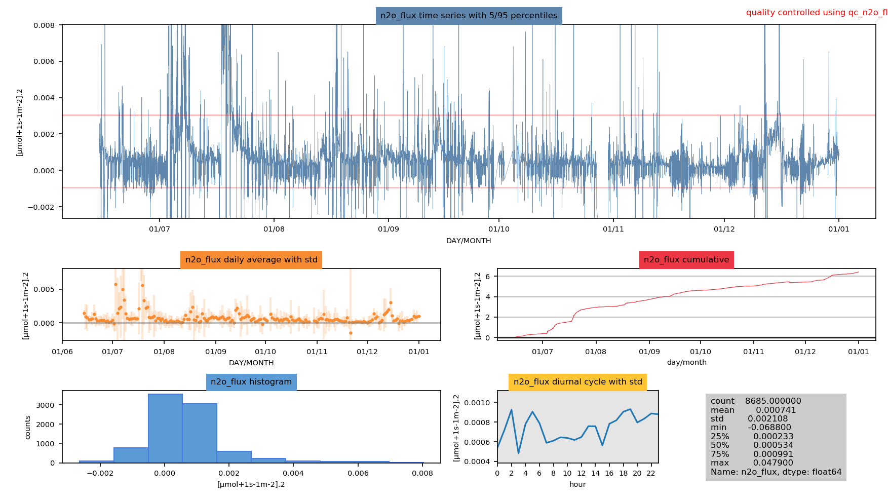
- The N2O flux looks like this:

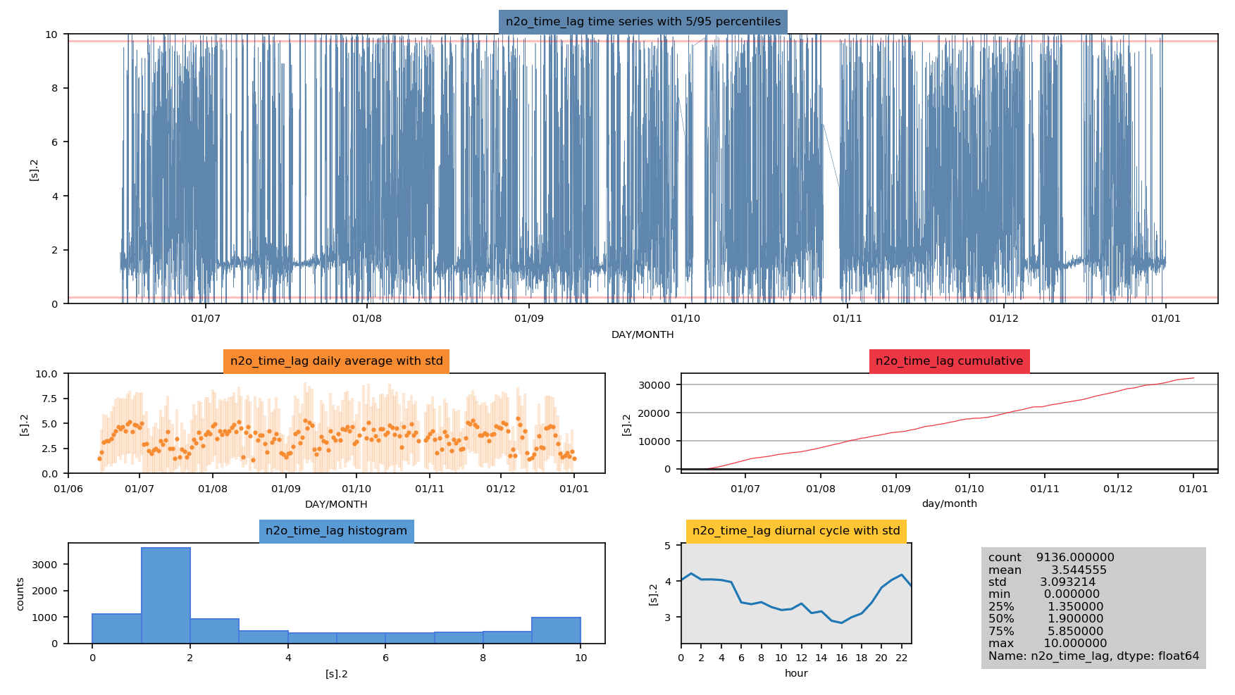
- Now let’s take a look at the found lag times:

- For many time periods, no clear lag could be found, but during certain time periods the maximum covariance was found consistently between 1-2s. This can be seen in the full time series plot, but also in the histogram (there is a peak between 1-2s). This indicates that the true lag is most likely in this range.
- For the final flux calculations (Level-1), the lag can be searched in a much smaller time window. Since we now know that the true lag in this example is most likely between 1-2s, the time window for the final flux calculations can be set to 0-5s.
- In EddyPro, we can also define a nominal lag time (also called default lag time), which is used in case no clear covariance peak can be found within the search time window.
- Looking at the distribution of found lag times in more detail, the peak of the distribution seems to be 1.45s. This value can be defined as nominal lag time in EddyPro.
Different scalars might have different peak times. For example, the lag time for H2O is generally longer than for CO2 in closed-path gas analyzers.
Last Updated on 19 Feb 2024 21:48